Journal of the Operations Research Society of Japan
Vol. 25, No. I, March 1982
Abstract
'AN EPQ MODEL FOR DETERIORATlNG
ITEMS UNDER LIFO POLICY
Hark Hwang
Korea Advanced Institute of Science and Technology
(Received March 16, 1981; Final October 2, 1981)
Inventory level in production quantity model has been developed for items that deteriorate contin· uous1y in accordance with a general probability distribution under Last In First Out (UFO) issuing policy. From the result developed, the earlier model by Misra for constant rate of deterioration can be obtained as a particular case. An approximate formula is derived using perturbation techniques. To illustrate the use of the formula an example problem is solved and an approximate optimum production quantity is found.
1. Introduction
A deteriorating product is one whose gradual loss of potential or utility is associated with the passage of time such as grain, photographic film, electronic components and radio-active material. Recently many inventory models have been considered in which inventory is depleted not only by physi-cal depletion but also by deterioration. The first attempt on this subject was made by Ghare and Schrader [3] who determined economic order quantity and
this model was extended to weibull distribution deterioration by Covert and Philip [2] and was further extended to the case of general distribution deteri-oration by Shah [8]. Cohen [1] considered the problem of simultaneously set-ting price and ordering quantity.
Nahmias and Wang [5] considered (Q,r) inventory system for item which is subject to continuous exponential decay and Nose, Ishii, Nishida and Hamada [6] extended it to the situation in which procurement lead time is treated as a finite varying stochastic variable. For a production quantity model, Shah and Jaiswal [9] considered a model in which backlogging is permissible with a constant deterioration rate and Misra [4] used a variable rate of deteriora-tion by assuming a two parameter Weibull distribudeteriora-tion. But the solution obtained by Misra is only correct for the case of constant rate of
deterioration. When the rate of deterioration is variable, the items whieh have entered inventory at different times have a different rate of deteriora-tion since the amount deteriorated during a given time interval depends on how long an item has been in stock. With an EOQ model with weibull distribu-tion deterioradistribu-tion eonsidered by Covert and Phi1ip [2] and Phi1ip [7], it is assumed that all items in one order enter the inventory at same time, so t:he above complexity does not occur.
In this article, inventory level for an Economic Production Quantity model with Last In First Out (LIFO) issuing policy for demand with items that deteriorate eontinuously in accordance vdth a general probability distribution for the lifetime of an item is developed. From the general model developed here, the result by Misra can be obtained as a particular case by taking an exponential distribution for the time to deterioration of an item.
2.
Development of the Model
Following is the list of assumptions we make to develop the model; (1) demand rate A is known and constant
(2) production rate P governing supply is finite and constant
(3) units are available for satisfying demand after their production (4) a deteriorated unit is not repaired or replaced
(5) the production rate P is greater than the demand rate (6) shortages are not allowed
(7) the number of units is treated as a continuous variable
(8) the time for an item to deteriorate follows
probability density function
(p.d.f.) f(t) (t
2:
0) andcwnulative distribution function (c.d.f.)
F(t)=l-R(t);
so that, the instantaneous deterioration rate of an item isD(t)=f(t)/(l-F(t»
=
f(t)/R(t), t
~o.
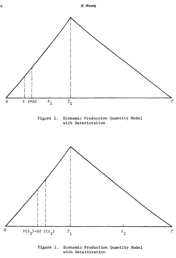
(9) Last In First Out (LIFO) principle Ls applied in satisfying demand. Figure 1. shows an inventory cycle for a finite production rate where T is a cycle time.
During time interval
(t, t+ t:, t)
wheret.s. T
1 produc tion occurs at a constant rate of P units per unit time and demand occurs at a constant rate of A units per unit time, leaving (P-A) ,~t to enter the inventory system due to LIFO policy.At time
tl
wheret.s. t1
.s. T1, the quantity (P-A)t:,t
which entered the inventory during(t,t+ t:,t)
reduced to(P--A)R(t
1
-t) t:,t
due to deterioration process shown in Fig. 1.50 H. Hwang
Figure 1. Economic Production Quantity Model with Deterioration
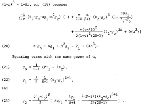
Figure 2. Economic Production Quantity Model with Deterioration
This gives the inventory level at time
t
1,It
1 as follows t (1) It =/1(p->-)R(t 1-t)dt. 1 0• During time interval (tz,tZ+~tZ) where T1
2
tz2
T, there is no produc-tion and demand during this interval is >-~tz which is satisfied from the inventory accumulated during (O,T1). Assume that the demand >-~tz is satisfied with the items produced during (t(t
Z) - ~t, t(tZ
»
shown in Fig. Z. Notice that at time tz the item produced during
(t(t
Z
),T
1
)
is not in the inventory system because they already satisfied the demand occured during(t(tZ),t
Z) due to LIFO principle. The above argument gives
(Z)
Therefore,
(3) -(P->-)R(tz-t).
If R(t) is known, t(t
Z) can be found from eq. (3) with initial condition, t=T
l at tZ=Tl due to LIFO policy and It becomes
2 (4) t(t
z)
/ (P->-)R(tZ-y)dy. o3. Case
From the general inventory level developed above, two particular cases are considered by taking the exponential distribution and the Weibu1l distri-bution for the time to deterioration of an item.
3.1. Exponential distribution for the time to deterioration of an item
Let the p.d.f. of the time to deterioration of an item be
f(t)
= a exp(-at) ,°
t ~ 0, a >
°
otherwise.
For this distribution R(t), D(t) are R(t) = exp(- at) and D(t) = a. With substitution of exp(- a(t
1-t» into R(t1-t) of eq. (1) and integration of the resultant equation, we obtain
52 (5) It 1 HHwang
P-A
= -
(l-exp(-at » a 1Similarly, from eqs. (3) and (4)
(6) It
=
-U-
P-A
exp(-at2) (exp(at)-l), 2 and (7) dt 2 A
d t
= -(P-A) exp(-a(t 2-t».The solution of eq. (7) with the boundary condition, t=T
l at t2=Tl is
(8) (P-A) exp(at) = P exp(aT
l) - A exp (at2). Substituting eq. (8) into eq. (6) yields
(9) It =
~
[P • exp (a(Tl-t2» - A - (P-A) exp (-at2)]. 2
We can show that our results are the same as those obtained by Misra but need to recognize that the origin of t2 in his formulation is at the end of t
l, Tl while that of tl and t2 in this article have a C01lUllon origin at the beginning of a cycle, that is t2 is equivalent to (T
l+t2) of Misra. In case of a constant rate of deterioration, the LIFO issuing policy does not have any effect On the inventory level.
3.2. Weibull distribution for the time to deterioration of an item
Assume that the p.d.f. of the time "to deterioration of an item isf(t) aStS-l exp(-at S)
o
t > 0
otherwise,
a > 0,
S
> 0where a,S are some constants determined by the deterioration process. For this distribution R(t), D(t) are
R(t)
=
exp(-atS) and D(t) Then, It and It become1 2 (10) It f tl (P-A) exp(-a(tl-t)S)dt, 1 0 and (11) It t (t 2) (P-A)
S
f exp(a(t 2-y) )dy, 2 0where
(12) >.. - - = - (p->..) exp (-a(tdt 2
6
2-t) ). dtTo solve eq. (12), let
(13) a (t
2 - t)6
=
x.
Substituting eq. (12) into the result obtained from differentiation of
eq. (13) yields
1 6-1
(14) a
S
6X-SC>"-P exp(-X)-l) dX>.. dt ,
and with the boundary condition, at t
2-2'1' t=T1 which in turn implies, at
t=T
1,X=0, the solution of eq. (14) is
(15) 1 6-1
S
-6- P->.. -1 J 0 [a 6y (1+ ->..- exp ( -y ) ) ] dy + T 1. x3.3. Approximation
We notice that solving eq. (15) with respect to t(t
2) seems to be very difficult because it is a transcendental equation. One way to obtain an approximate solution of t(t
2) is to solve eq. (12) under the assumption that
0.« 1. The validity of this assumption and physical meaning of a when 13=1. is explained in detail by Ghare and Schrader
[3].
Let u=t
2-t and v=P->... Then eq. (12) becomes
(16) A(dU
+
1)dt
i3 -v exp (-o.u ),
and the solution of eq. (16) with the boundary condition, at u=O, t=T l, is
(17) u -A du'
J 0 >.. + exp(-au,6)v
Using the series form of the exponential and ignoring terms with third and higher order powers of a, eq. (17) becomes
->..u S 2 213 0(0.3)] (18) Hv [ 1. + v au + v(v->..)a u +
=
t-Tl• >"+v S+l 2(Hv)2(2S+l) Let t=go+ agl (t2) + a 2 g2(t 2) + 0(0. 3 ), then u becomes (19) U = t2 - g - "'gl - a2g 2+
0(0. 3 ). o v.54 H. Hwang
Substituting eq. (19) into eq. (18) and using approximation formula,
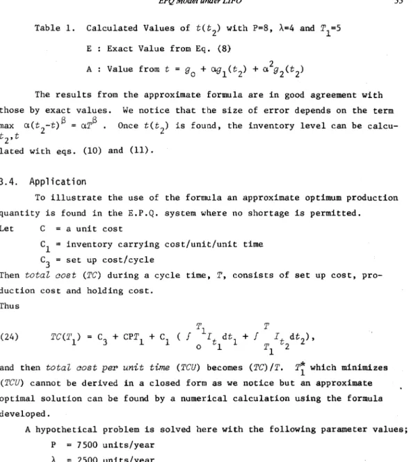
(l-x) 13 = 1-13x, eq. (18) becomes (20) (21) (22) and (23) a 13 aSg 1 1
+
~ A+V 13+1 (t2-g0) (1- - - ) t 2-go
2 + v(v-A)a (t _g )213 + 0(a3)] 2 (A+V) 2(213+1) 2 0 2 3 = go+
agl
+
a g2 -Tl
+
O(a ). Equating terms with the same power of a,g =
2
A(P-2A) (t
2
-g
o) 13+12P(2(3+1) ]
With this perturbation technique, it is theoretically possible to obtain an approximate value of t to any desired accuracy using higher powers of a. Table 1 is the tabulated results of t(t
2) from example problems to compare 2
the approximate formula of t(t2), t(t2) = go + agl(t2) + a g2(t2) where gi(t2) is defined as eqs. (21), (22) and (23) respectively with the exact values calculated from eq. (8) when (3 = 1.
~
a=O.l 13=0.1 a=O.l 13=0.5 a=O.l (3=1. 5t2 E A A A 5.0 5.0000 5.0000 5.0000 5.0000 5.5 4.4737 4.4731 4.4647 4.4781 6.0 3.8888 3.8850 3.8979 3.8565 6.5 3.2346 3.2244 3.3093 3.0343 7.0 2.4974 2.4800 2.7022 1,8736 7.5 1. 6589 1.6406 2.0787 0.1945 8.0 0.6943 0.6950 1.4401
-8.5-
-
0.7874 -9.0-
-
0.1213 -cycle time 8.3180 8.3333 9.0900 7.5476Table 1. Calculated Values of t(t
2
)
with P=8, A=4 andT
l
=5
E Exact Value from Eq. (8)A
The results from the approximate formula are in good agreement with those by exact values. We notice that the size of error depends on the term max CI.(t
2-t)S
=
Cl.TS .
Once t(t2) is found, the inventory level can becalcu-t
2,t
lated with eqs. (10) and (11).
3.4. Application
To illustrate the use of the formula an approximate optimum production quantity is found in the E.P.Q. system where no shortage is permitted.
Let C a unit cost
Cl inventory carrying cost/unit/unit time C
3 set up cost/cycle
Then total oast (TC) during a cycle time, T, consists of set up cost, pro-duction cost and holding cost.
Thus (24) TC(Tl)
=
C 3+
CPTl+
Cl( !
Tl T dt2), It dt l+!
It 0 1 T1 2and then total oast per unit time (TCU) becomes (TC) /T. T~ which minimizes (TCU) cannot be derived in a closed form as we notice but an approximate optimal solution can be found by a numerical calculation using the formula developed.
A hypothetical problem is solved here with the following parameter values; P 7500 units/year A 2500 units/year Cl. 0.2
a
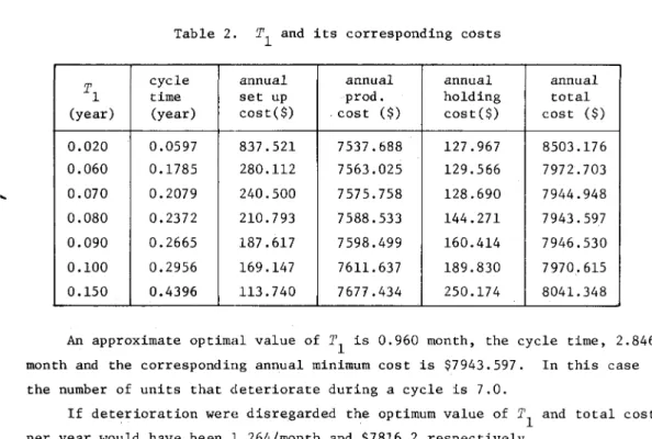
1.2 C $3.00/unit Cl $0.60/unit/year C 3 $50.00/set up.For each value of Tl chosen, cycle time, annual set up cost, annual pro-duction cost, annual holding cost and annual total cost (TCU) are calculated and Table 2, shows part of the results.
56 H. Hwang
Table 2. Tl and its corresponding costs
Tl cycle time annual set up annual prod. holding annual annual total (year) (year) cost($) cost ($) cost($) cost ($)
0.020 0.0597 837.521 7537.688 127.967 8503.176 0.060 0.1785 280.112 7563.025 129.566 7972.703 0.070 0.2079 240.500 7575.758 128.690 7944.948 0.080 0.2372 210.793 7588.533 144.271 7943.597 0.090 0.2665 187.617 7598.499 160.414 7946.530 0.100 0.2956 169.147 7611.637 189.830 7970.615 0.150 0.4396 113.740 7677.434 250.174 8041.348
An approximate optimal value of Tl is 0.960 month, the cycle time, 2.846
month and the corresponding annual minimum cost is $7943.597. In this case the number of units that deteriorate during a cycle is 7.0.
If deterioration were disregarded the optimum value of Tl and total cost
per year would have been 1.264/month and $7816.2 respectively.
4.
Conclusion
Inventory level in a production quantity model for items that deteriorate continuously in accordance with a general probability distribution has been qeveloped. In case of a variable rate of deterioration, complexity arises due to the fact that the amount deteriorated during a given time interval depends on the time item has entered the inventory. To solve this difficulty we assume the inventory manager select Last In First Out (LIFO) as an issuing policy. Weibull and exponential distribution for the time to deterioration of an item are considered. With constant rate of deterioration, the result developed is shown to be consistent with the Misra's.
Due to difficulty in solving t(t
2) in eq. (15), an approximation formula
using perturbation techniques is developed and is illustrated its usage through a example problem.
References
[1] Cohen, M. A.: Joint Pricing and Ordering Policy for Exponentially
Decaying Inventory with Known Demand, Naval Research [~gistics Quarterly, Vol.24, No.2 (1977).
[2] Covert, R. P. and Philip, G. C.: An EOQ Model for Items with Weibull Distribution Deterioration, AIIE Transactions, Vol.S, No.4 (1973). [3] Ghare, P. M., and Schrader, G. F.: A Model for Exponentially Decaying
Inventories, Journal of Industrial Engineering, Vol.14, No.S (1963). [4] Misra, R. B.: Optimum Production Lot: Size Model for a System with
Deteriorating Inventory, International Journal of ~oduction Research, Vol.13, No.S (1973).
[S] Nahmias, S., & Wang, S. S.: A Heuristic Lot Size Reorder Point Model for Decaying Inventories, Management Science, Vol.2S, No.l (1979).
[6] Nose, T., Ishii, H., Nishida, T., and Hamada, A.: Decaying Inventory Problem Subject to Stockout Constratnt, Technological Report of Os aka University, Vol.30 (1980).
[7] Philip, G. C.: A Generalized EOQ Model for Items with Weibull Distribu-tion DeterioraDistribu-tion, AIIE Transactions, Vol.6, No.2 (1973).
[8] Shah, Y. K.: An Order-Level Lot-Size Inventory Model for Deteriorating Items, AIIE Transactions, Vol.9, No.l (1977).
[9] Shah, Y. K., and Jaiswal, M. C.: A Lot-Size Model for Exponentially Deteriorating Inventory with Finite Production Rate, Gujarat StatistiClaZ Review, Vol.3, No.2 (1976).
Hark HWANG: Associate Professor Dept. of lE, Korea Advanced
Institute of Science and Technology P.O. Box ISO, Chongryang