Optimization Based Globally Convergent Methods for the Nonlinear Complementarity Problem

(1)

Society of Japan

VoJ. 37, No. 4, December 1994

OPTIMIZATION BASED GLOBALLY CONVERGENT

METHODS FOR THE NONLINEAR COMPLEMENTARITY PROBLEM

Kouichi Taji Masao Fukushima Nara Institute of Science and Technology

(Received June 14, 1993; Revised January 28, 1994)

Abstract The nonlinear complementarity problem has been used to study and formulate various equi-librium problems including the traffic equiequi-librium problem, the spatial equiequi-librium problem and the Nash equilibrium problem. To solve the nonlinear complementarity problem, various iterative methods such as projection methods, linearized methods and Newton method have been proposed and their convergence re-sults have been established. In this paper, we propose globally convergent methods based on differentiable optimization formulation of the problem. The methods are applications of a recently proposed method for solving variational inequality problems, but they take full advantage of the special structure of nonlinear complementarity problem. We establish global convergence of the proposed methods, which is a refinement of the results obtained for variational inequality counterparts. Some computational experience indicates that the proposed methods are practically efficient.

1. Introduction

We consider the nonlinear complementarity problem, which is to find a vector x E Rn such that

:c ~ 0, F(x) ~

°

and xT F(x) = 0, (1)

where F( x) = (Fl(X), F2(x), ... , Fn(x))Y is a given continuously differentiable mapping from Rn into itself and T denotes transposition. This problem has been used to formulate and

study various equilibrium problems including the traffic equilibrium problem, the spatial economic equilibrium problem and Nash equilibrium problem [1,6, 13, 15, 18].

To solve the nonlinear complementarity problem (1), various iterative algorithms, such as fixed point algorithms, projection methods, nonlinear Jacobi method, successive over-relaxation methods and Newton method, have been proposed [8, 10, 16]. Many of these methods are generalizations of classical methods for systems of nonlinear equations and their convergence results have been studied extensively [10, 16].

Assuming the monotonicity of mapping F, Fukushima [7] has recently proposed a differ-entiable optimization formulation for variational inequality problem and proposed a decent algorithm to solve variational inequality problem. Based on this optimization formulation, Taji et al. [17] proposed a modification of Newton method for solving the variational in-equality problem, and proved that, under the strong monotonicity assumption, the method is globally and quadratically convergent.

In this paper we apply the methods of Fukushima [7] and Taji et al. [17] to the nonlin-ear complementarity problem. We show that those methods can take full advant.age of the special structure of problem (1), thereby yielding new algorithms for solving strongly mono-tone complementarity problems. We establish global convergence of t.he proposed methods, which is a refinement of the results obtained for the variational inequality count.erparts in several respects. In this paper we show that the compactness assumption made in [7] can

(2)

be removed for the strongly monotone complementarity problem. Moreover, some computa-tional results shows that the proposed met.hods are practically efficient for solving monotone complementarity problems, though the convergence of the proposed methods is theoretically proved only under the strong monotonicity assumption.

2. Equivalent optimization problem

In this section, we introduce a merit function for the nonlinear complementarity problem (1) and present some of its properties.

Choose positive parameters 5i

>

0, i = 1,2, ... , n and define the function

f :

Rn ... R

by

~

1 {

2 2}

f(x)

=:Si

25

i Fi(X) - (max(O, Fi(X) - 5iXi)) . (2)

This function is a special case of the function originally introduced by Fukushima [7] for variational inequality problem. Though, some of its properties can be derived from the results of [7], we give here simple and direct proofs for these properties, which utilize the special struct ute of problem (1).

For convenience, we define

(3)

n

hence f is written as f(x) =

L

f;(x). We denote D as a diagonal matrix such that i=1

D = diag(51 , 52,,'" 5n ), and ei as the i-th unit vector such that

o

ei = 1

<

i.

o

We also denote

M(x)

=

max(O, x --D-1 _F(x)),

₍₄₎

where max operator is taken component-wise, i.e.,

Mi(X) = max(O, Xi -

5;1

Fi(X)).

Using this notation, we have the following result.

Lemma 1 Let the mapping M : Rn - t R~ be defined by (4). Then x* solves (1) if and only if x* = M(x*).

Proof. Suppose that x* is a solution to (1). Then either

holds for all i = 1,2, ... , n. Since 5i

>

0, we have

(3)

and

Fi{:r*)

=

0 ===? Mi(X*)

=

max(O,

x7)

=

x:.

Thus Mi(X*) = xi for all i.

On the other hand, suppose that X* satisfies x* = M{ x*). Then, for all i, either

{ *

x· 1.

=

0

{* *

x· t

=

x· - v· t --IF ( 1. t . X

*)

x* - 8:-1 _P(x*)

_<

₀ _or x~ _{- D:-1p(x*)}

_>

₀

t 1. 1. _ t t t _

holds. Hence, it follows from (ji

>

0 that either x; = 0 and Fi{X*) ;::: 0, or xi ;::: 0 and

Fi{X*)

=

0 holds for all i. Thus X* solves (1). 0

Using the function (2), an equivalent optimization problem is obtained for nonlinear corn plementarity problem (1).

Proposition 1 Let the function f : Rn --t R be defined by

(2).

Then f{x) ;:::

0

for all

x ;::: 0, and f(x) = 0 if and only if x solves (1). Hence, x solves (1) if and only if it is a solzttion to the following optimization problem and its optimal value is zero:

minimize f{x) subject to x;:::

o.

(5)

Proof. We first show that /;(x) ;::: 0 for all x ;::: 0, so that f(x) ::::: 0 for all x ::::: O. If

Fi(X) - DiXi :::; 0, then fi(X)

= (2Di)-1 Fi(X)2 ;:::

O. So we consider the case Fi{x) - DiXi

>

O. Since Di

>

0, Xi

2::

0 and Fi(X)

>

DiXi hold, we see, from (3),

fi(X)

2~.

{Fi(X)2 - (Fi(X) - Di Xi)2}

,

Di 2 XiFi(X) -

2

Xi (ji 2

>

-x·

2 '

>

O.

Therefore,

f

(x) ::::: 0 for all x ;:::

o.

Next, suppose f(x) = O. Then f;(x)

=

0 must hold for all i. Hence, as shown in the above, either Fi{x)

=

0 and Fi(X) - DiXi :::; 0, or Xi

=

0 and Fi(X) - DiXi

>

0 holds for all i.

Therefore, x is a solution of (1).

On the other hand, suppose that x solves (1). Then either F{Xi) = 0 or Xi == 0 holds for all i. If F(Xi)

=

0, then from (3) we have

Also if Xi = 0, then we have

Therefore, f(x) = O.

1 2

fi(X) = - 2Di (max{O, -DiXi)) = O.

=

~{Fi(X)2

- (max(0,Fi(X)))2}

28i

=

2~i

{Fi(X)2 - Fi{X)2}

= O.

(4)

Remark 1 When problem (1) has no solution .. the optimization problem (5) may have a minimizer which does not zero the function

f.

For example, let consider the case RI and

F(x) = -x - 1. Clearly, the complementarity problem has no solution. On the other hand, given {j

>

0, the corresponding optimization problem (.5) is formulated as

1

minimize -(x

+

1)2 subJ'ect to x

>

0.

2{j

-The unique optimal solution to this problem is X' = 0, at which the function value is 21{j

>

0. It can be shown that the function 1 is continuously differentiable whenever so is the mapping F.

Proposition 2 If the mapping F is continuously differentiable, then so is the function f defined by (2), and the gradient of

1

is given by

V'/(x) = F(x) - (V' F(:r) - D)(M(x) - x). (6)

Proof. We first note that, if a function B : Rn - t R is continuously differentiable and 0( x) = (max(O,

B(

x)))2, then 0 is continuously differentiable and the gradient of 0 is given by

V'0(x) = 2 max(O, B(x))V'B(x).

Hence, from (3) we have

1

V'/i(X) = '6.(Fi(x) - max(O, Fi(X) - {jiXi))V' Fi(X)

+

max(O, F;(x) - {jixi)ei. (7)

,

Since

max(O, Fi(X) - {jixd F;(x) - {j,iXi

+

{ji max(O, Xi - {j;-1 Fi(X)) Fi(X) - {j,iXi

+

{jiMi(X)

holds, we have from (7)

V' f;(x) '8;(Fi(x) -1 max(O, F;(x) - {ji;Z;i)) V' Fi(X)

+

max(O, F;(x) - {jixi)ei (Xi ~ Mi(X))V' Fi(X)

+

(Fi(X) - {jiXi

+

{jiM;(x))ei.

Therefore, we have from (8) n

V'/(;z;) = LV' j;(x)

i=l n

L

{(Xi - M;(x))V' Fi(X)

+

(Fi(X) - {jiX;

+

{j;Mi(x))e;}

;=1

F(x) - (V' F(x) - D)(M(x) - X).

(8)

o

Proposition 1 says that finding a global optimal solution to (5) amounts to solving the complementarity problem (1). However, in general, optimization algorithms may only find a stationary point of the problem. Thus it is desirable to clarify conditions under which any stationary point of problem (5) actually solves problem (1). The next proposition answers for this question.

(5)

Proposition 3 Suppose that V' F( x) is positive definite for all x

2':

o.

If x

2':

OIS a station-ary point of problem (5), i.e"

(y - x)TV' f(x)

2':

0 for all y

2':

0, (9) then x is a global optimal solution of problem (.5), and hence it solves the nonlinear comple-mentarity problem (1).

Proof. Suppose that x satisfies (9). Then from (6) we have

(M(x) - xfV' f(x)

(M(x) - xf {(F(x) - Dx

+

DM(x)) - V' F(x)(M(x) - xl}

= (M(x) - xf(F(x) - Dx

+

DM(x)) - (M(x) - x)TV' F(x)(M(x) - x). (10) It is easy to see that

(M(x) - x)T(F(x) - Dx

+

DM(x))

n

L{8;(max(0,x; - 8;lF;(x)) - Xi?

+

(max(O,x; - 8;-lFi(X)) - x;)F;(x)}

;=1

<

O. (11 )

Since

x

satisfies (9), it follows from (10) and (11) that

(M(x) - xfV' F(x)(M(x) - x) ::; O.

However, since V' F(x) is positive definite, we have x = M(x). Therefore, it follows from

Lemma 1 that x is a solution to (1). 0

We say that the mapping F is strongly monotone on R~ with modulus JL

>

0, if

(x - yf(F(x) - F(y))

2':

JL 11 x - y 112 for all x, y

2':

O.

(12)

The following result establishes an asymptotic behavior of the function

f.

Note that similar results have not been obtained for variational inequality problems.

Proposition 4 If F is strongly monotone on R~, then

lim f(x) =

+

00.

"'~O, 11"'11->00

Proof. Let {xk} be a sequence such that xk

2':

0 and 11 xk 11---+ 00. Taking a subsequence if

necessary, we may suppose that there exists a set I C {I, 2, ... ,

n}

such that

x7

---+ +00 for

i E I and {x7} is bounded for i ~ I. From {xk}, we define another sequence {yk} such that

yf

= 0 if i E I and

yf

=

xf

if i

rf.

I. From (12) and the definition of

yk,

we have

( 13)

iEI iEI

By Cauchy's inequality we have

1 1

(L(Fi(x k

) - F;(yk))2) 2" (L(X

7 ?)

2"

2':

L(Fi(Xk) _ Fi(yk))x7- (14)

(6)

It then follows from (13) and (14) that

(15)

iEI iEI

Since {yk} is bounded by definition, {Fi(yk)} is also bounded. Therefore, since x7 ---t

+00

for all i E I, (15) implies

iEI

As shown at the beginning of the proof of Proposition 1, j;(xk) =

~Fi(Xk)2

>

0 if

28i

8· F;(xk

) - 8;x7 :::; 0, and fi(xk) :::: i(x7)2 if Fi(X k ) - 8ix7

>

o.

Therefore we have n f(x k)

L

fi(xk) i=l

>

L

fi(xk) iEI

>

L

2~.

min(Fi(xk)2, (oi x7?)· ;EI •

Since x7 ---t

+00

for all i E I and

L

Fi(X k)2 ---t x>, it follows that f(x k) ---t

+00.

0

iEl

3. Algorithms

In this section, we propose two globally convergent methods for solving (5). One is based on the methods of Fukushima [7] and the other the method of Taji et al. [17], which were originally proposed for variational inequality problems. Throughout this section, we suppose that the mapping F is strongly monotone on R~ with modulus 11

>

o.

3.1. Descent method

The first method uses the vector

d M(x) - x

max(O, x - D-1 _{F(x)) - x} ₍₁₆₎

as a search direction at x. When the mapping F is strongly monotone, it can be shown that the vector d given by (16) is a descent direction.

Lemma 2 If F is strongly monotone with modulus 11, then the vector d given by (16) sat-isfies the descent condition

Proof. From (10) and (11), we have

(M(x) - xfY' f(x) :::; -(M(x) - x)TY' F(x)(M(x) - x). ( 17)

It is known that, when F is differentiable and strongly monotone on R~, Y' F satisfies

(7)

Therefore, from (17) we have

o

Thus the direction d can be used to determine the next iterate by using the following Armijo-type line search rule: Let a := /Tn, where

m

is the smallest non negative integer 171

such that

f(x) - f(x

+

rrd)

2:

air 11 d 112,

where 0

<

(3

<

1 and a

>

O. Note that, in the descent method originally proposed by Fukushima [7] for variational inequality problems, the line search only examines step sizes shorter than unity. Here, we propose the algorithm that allows longer step sizes at each iteration.

Algorithm 1:

Choose XO

2:

0, a

>

1, (3.::: (0,1), a> 0 and a positive diagonal matrix D; k:= 0

while convergence criterion is not satisfied do

dk:= max(O,xk - D-1P(Xk_{)) -} _Xk;

i:=

max{t 1 xk

+

tdk

2:

0, t

2:

O}; m :=0 if f(xk ) - f(xk

+

dk)

:2'

a 11 dk 112 then else while am

:s

i and

f(xk ) - f(xk

+

amdk)

2:

aam 11 dk 112 and f(x k

+

am'Hdk )

:S

f(x k

+

amdk) do m:=

m+

1 endwhile xk+l := xk

+

amdk while f(x k) - f(xk

+

_(3mdk )

<

a(3m 11 dk ₁₁₂ _do m:=

m+

1 endwhile Xk+l := xk

+

(3mdk endif k := k

+

1 endwhile

Note that the vector M(xk+l) = max(O,xk+l - D-1P(Xk+l)) has already been found at the previous iteration as a by-product of evaluating

f.

Therefore one need not compute again the search direction dk _{at the beginning of each iteration.}

Theorem 1 Suppose that the mapping P is continuously differentiable and strongly mono-tone with modulus J-l on R~. Suppose also that V' P is Lipschitz continuous on any bounded subset of R~. Then, for any starting point xO

2:

0, the sequence {xk} generated by Algorithm

1 converges to the unique solution of problem

(1)

if the positive constant a is chosen to be sufficiently small such that (T

<

J-l.

Proof. By Proposition 4, the level set S = {x 1 f(x)

:S

f(xO)} is bounded. Hence V' P is

(8)

is also Lipschitz continuous on 5. Under these conditions, it is not difficult to show that

\7

f

is Lipschitz continuous on 5, i.e., there exists a constant.

L

>

0 such that 11 \7

f(x) -

\7

f(y)

11::;

L

11

x -- y

11 for all

x,

yE 5.

Therefore, as shown in the proof of [7, Theorem 4.2], any accumulation point of

{xk}

satisfies

x

=

M(x),

and hence solves (1) by Lemma 1. Since strong monotonicity of

F

ensures that problem (1) has a unique solution, we can conclude that the entire sequence converges to

the unique solution of (1). 0

Remark 2 In Fukushima [7], global convergence theorem assumes not only the strong monotonicity of mapping F but the compactness of the constraint set, which is not the case for nonlinear complementarity problems. Theorem 3.1 above establishes global convergence under strong monotonicity of the mapping F onl.y.

3.2. Modification of Newton method

The second method is a modification of Newton method, which incorporates a line search strategy. The original Newton method for solving the nonlinear complementarity problem (1) generates a sequence {Xk} such that XO

2:

0 and Xk+l is determined as Xk+l :=

x,

where

x

is a solution to the following linearized complementarity problem:

It is shown [16] that, under suitable assumptions, the sequence generated by (18) quadrat-ically converges to a solution x' of the problem (1), provided that the starting point .ro is chosen sufficiently close to x'.

Lemma 3 When the mapping F is strongly monotone with modulus J.l, the vector dk :=

x -

xk

obtained by solving the linearized complementarity problem (18) satisfies the inequality

Therefore, dk _{is actually a feasible descent direction of f at}_Xk,_{if the matrix D is chosen to}

satisfy 11 D 11= max(8;)

<

4J.l .

•

Proof. For simplicity of presentation, we omit the superscript k in xk and dk. Since

d :=

x -

x, it follows from (6) that

\7f(xfd

(x - x)T F(x)

+

(x - x)T(,\7 F(x) - D)(x - M(x))

(x - xf(F(x)

+

\7F(xf(j; - x)) - (x - x)T\7F(x)T(X - x))

+(x - M(x))T(F(x)

+

\7

F(x)T(x - x))

-(x - M(x)f F(x) - (x -

xf

D(x - M(x))

-(M(x) - xf(F(x)

+

\7

F(x)T(x - x))

+(M(x) - X)T F(x)

+

(x -

xf

D(M(x) - x)

-(x - xf\7 F(xf(x - x).

( 19)

Since

x

is a solution to (18) and M (x)

2:

0, the first term of (19) is nonpositive. From (11), we have

(9)

Then it follows from the second term of (19) that

(M(x) -

xf

F(x)

+

(x -

xf

D(M(x) - x)

<

(x -

xf

D(M(x) - x) - (M(x) - x)T D(M(x) - x)

n

L

8i{(Xi - xi)(Mi(X) - Xi) - (Mi(X) - Xi?}

i=l

n 8.

L

i{(Xi - Xi? - (Mi(X) - Xi)2 - (Xi - Mi(X)?}

i=l

~

8i _{

)2

_{1 (}

2}

<

~"2 (Xi - Xi

-"2

Xi - Xi)

~

8i

₎₂

L4(Xi - Xi i=l 1

=

-(x --X)T D(x - x). 4

Hence, we have from (19) and (20)

V f(xf d :::; -dTV F(xf d

+

~dT

Dd.

(20)

But since strong monotonicity of F implies dTV F( x)d

2':

J.L 11 d 112 and since dT Dd :::; 11 D 11 11 d 112, we have

\If(xfd

< -

(J.L -

~

IIDII) Ild112.

The last half of the proposition then follows immediately. 0

Using this result, we can construct a modified Newton method for solving the nonlinear complementarity problem (1).

Algorithm 2:

Choose xO

2':

0, j3 E (0,1), a E (0, ~), and a positive diagonal matrix D; k:= 0

while convergence criterion is not satisfied do

find xk such that

Xk

2':

0, F(Xk)

+

V F(xkf(Xk - xk)

2':

0 and (xk)T(F(x k)

+

V F(xk)T(xk _- _xk))

₌

_0; dk := xk _ xk; m:=O while f(xk_{) --} _f(xk

₊

_j3mdk₎

_<

_-aj3mVf(xk?dk _do m:=

m+

1 endwhile xk+1 _:=_xk

+

_{j3mdk ;} k := k

+

1 endwhile

When the mapping F is strongly monotone, we can establish the global convergence of Algorithm 2.

Theorem 2 Suppose that the mapping F is continuously differentiable and strongly mono-tone with modulus J.L. If the matrix D is chosen such that 11 D 11 = max( 8;)

_,

<

4J.L, then,

(10)

for any starting point XO

2::

0, the sequence {xk} generated by Algorithm 2 converges to the solution of (1).

Proof. By Lemma 3 and the Armijo line search rule, the sequence {f( xk)} is nonincreas-ing. It then follows from Proposition 4 that the sequence {xk} is bounded, and hence it contains at least one accumulation point. As shown in the proof of [17, Theorem 4.1], any accumulation point of {Xk} is a solution of (1). Since strong monotonicity of F ensures that problem (1) has a unique solution, we can conclude that the entire sequence converges to

the unique solution of (1). 0

We can also show that the rate of convergence of Algorithm 2 is quadratic if F E: C2

and the strict complementarity condition holds at the unique solution x* of (1).

Theorem 3 Suppose that the sequence {xk} generated by Algorithm 2 converges to the solution x· to problem (1). Suppose also that the mapping F belongs to class C2

, V F( x·) is

positive definite and V2 _{F is Lipschitz continuous on some neighborhood of x*. If the drict}

complementarity condition holds at x·, i. e., x; = 0 implies Fi (x·)

>

0 for all i = 1, 2, ... , 71,

then there exists an integer

k

such that the unit step size is accepted for all k

2::

k.

Therefore, the sequence {xk} converges quadratically to the solution x* .

Before proving Theorem 3, we show the following lemma.

Lemma 4 Let x* be a solution to problem (1). If F E C2 _{and the strict complementarity}

condition holds at x*, then fi E C2 _{on a neighborhood of x*, and the gradient and the} Hessian of J; are given by

and

V

l( ) - {

(XiV Fi(x)

+

Fi(x)ei) - Dixiei if i E I*

,x - t,Fi(x)V Fi(X) if i E

1*

if i E /*

if i E

1*,

respectively, where I* =

{i

I

x; =

O}

and 1* =

{i

I

x;

>

O}.

(21a) (21b)

(22a) (22b)

Proof. The strict complementarity and the continuity of F ensure that there is a neigh-borhood B of x* such that

{ Fi (x)-6iXi>0 if i E /*

(23)

Fi(X) - 6iXi

<

0 if i E

1·

holds for all x E B. Hence, we have from (3)

1-( ) - { XiFi(X) -

%·x~

if i E /* (24a)

,x - -.LP(xf _if_i_E_1*. _(24b)

26, '

Therefore, by differentiating (24a) and (24b) directly, we have (21a), (21b) and (22a), (22b).

o

Proof of Theorem 3. It is sufficient to show that f(x k ) - f(x k )

2::

-(TV f(xkf(x k -- xk)

holds for sufficiently large k. For simplicity, we consider the case 61 = ... = 6n = 6

>

0, i.e.,

(11)

the result to the general case. Without loss of generality, we assume

J*

= {l, l

+

1, ... ,

n},

where 1

:s;

l

:s;

n, and denote

Since the strict complementarity holds at x*, there is an integer Kl such that ;rk satisfies if i E f*

if i E

J*

(25a) (25b) for all k ~ K1 . Under the given assumptions, Newton method (18) is locally quadratically

convergent to the solution :r* [16]. Hence, it follows from the strict complementarity and the continuity of F and V' F that there is an integer K2 such that

for all

k

~

K

2 • and and

Fi(X k)

+

V'

Fi(xkf(xk - xk)

>

0

Fi(X k)

+

V'

Fi(Xk)T(xk - xk)

= 0 if i E f* if i E

J*

(26a) (26b)

Now suppose k ~ max(}(l, K2)' For simplicity of presentation, we omit superscript kin

xk

and

xk.

For each i E 1*, we have

fi(X) - j;(x)

+

0"

V'

fi(xf(x - x)

(XiFi(X) -

~x~)

-. (XiFi(X) -

~x~)

+

O"(xiV' Fi(X)

+

Fi(x)ei - 8xieif(x - x)

8 2 T 2

XiFi(X) - 2Xi

+

O"(xiV' Fi(x) (x - x) - XiFi(X)

+

DXi )

>

xi.Pi(x) -

~X;

+

0"( -2XiFi(X)

+

8x;)

(1- 20") (XiFi(X) --

~X~)

>

(~-

0") 8x;

(~

- 0") 8(x; - Xi?,

(27)

where the first equality follows from (21a) and (24a), the second equality and the first inequality follow from (26a), the second inequality follows from (25a) and the last equality follows from (26a).

On the other hand, since by the mean value theorem we have

1

fi(X) - fi(X)

=

V'fi(xf(x - x)

+

2(x - X)TV'2fi(O(X - x)

for some ~ in line segment of x and

x,

we have

j;(X) - !i(X)

+

0"

V'

!i(xf(x - x)

1

(0" -

1)V'

!i(xf(x - x) - 2(x - X)TV'2 !i(O(X - x)

1

(0" -

1)V'

fi(xf(x - x) - 2(x - x)TV'2 j;(x)(x - x)

1

+-(x - xf(V'2!i(X) - V' 2fi(O)(X - x).

2 (28)

(12)

Then for each i E

t,*

we have

1

(0- -

1)V' fi(X)T(X - x) - 2(x - x)TV'2 fi(X)(X - x)

0--1

T I T 2 T

-15 -Fi(X)V' Fi(X) (x - x) - 2b(x - x) (F;(x)V' F;(x)

+

V' Fi(X)V' Fi(X) )(x - x)

1 (1)

T 2

1 .

T 2

8 2 -

0-

(V' Fi(X) (x - x)) - 28Fi(X)(x - x) V' Fi(X)(X - x)

=

~

G

-

0-)

(V' Fi(X*f(x - x)? - 21bFi(X)(x - XfV'2 Fi(X)(X - x)

+~ (~

-

0-)

(x - X)T(V' Fi(X)V' Fi(xf - V' Fi(X*)V' Fi(X*)T)(x - x), (29)

where the first equality follows from (21b) and (22b), and the second equality follows from (26b). Hence, we have from (28) and (29)

J;(x) - j'i(X)

+

o-V'fi(xf(x - x)

1 ( 1 ) T 2 1 T 2

=

8 :2 -

0-

(V' Fi(X) (x - x)) - 2SFi(x)(x - x) V' Fi(x)(x - x)

1

+2(X - Xf(V'2 fi(X) - V'2 fi(O)(X - x)

+~

G

-

0-)

(x - xf(V' Fi(X)V' Fi(X)T - V' Fi(X*)V' Fi(X*f)(x - x).

When V'2 F is Lipschitz continuous and is bounded on some neighborhood of x*, it is not difficult to show that V'2 fi and V' Fi are also Lipschitz continuous. Moreover, for i E

Y*

we have Fi(X) ~ 0 if x ~ x*. Hence, we have

J;(x) - J;(x)

+

o-V'fi(xf(x - x)

2:

~

G

-

0-)

(V' Fi(X*f(x - x)?

+

0(11 x - x* 11

+

11 x - x 11) 11 x - x 112 (30) holds on some neighborhood of x*.

Therefore, it follows from (27) and (30) that

f(x) - f(x)

+

o-V' f(xf(x - x)

>

8

(~-

0-)

L(Xi - Xi)2

+

~ (~-

0-)

L(V'Fi(xf(x - x)?

2 iEJ- 8 2

iEr-+0(11 x - x* 11

+

11 x - xii) 11 x - x 112

=

~

G

-

0-)

(x - xf A(x - x)

+

0(11 x - x* 11

+

11 x - xii) 11 x - x 112, (31) where A is a matrix such that

A = ₍15

2

El 0) (0 V'J-Fr-(x*)) ( 0

o

0

+

0 V'r-Fr-(x*) V'J-Fr-(x*f

( 8EI V'/_Fr-(X:)) (bEL V'1_Fr_(x:))T

_o

_{V'r- Fr- (x )} ₀ _{V'l- Fr- (x )}

where El is the I x I identity matrix. Clearly A is positive semi-definite. Moreover, since V' F( x*) is positive definite by assumption, the matrix V'r* Fr- (x*) is also positive definite.

H _{ence, t e matnx}h . (8EI V'/*Fr-(X*)). ₀ _{V'r- Fr- (x*)} _{IS nonsmgu ar , an}. 1 d h A ' _ence _{IS posItIve e mte.}.. d fi .

(13)

Remark 3 Taji et al. [17] have obtained a globally convergent Newton method for varia-tional inequality problems. In their method, to obtain quadratic convergence, the following line search procedure is used:

Let 0

<

(3

<

1, 0

<

I

<

1 and (J E (0,1); if f(x k

+

dk ) ~ If(x k ) then ilk := 1 else m:= 0 while f(x k ) - f(x k

+

(3mdk )

<

_(J(3mdkT

v

f(x k) do m:=

m+

1 endwhile ilk := (3m endif Xk+1 _:=_xk

+

_{ilk dk}

Note that this line search procedure, which is similar to the one used by Marcotte and Dussault [14], first checks if the unit step size is acceptable. On the other hand: Algorithm 2 employs Armijo rule in a more direct manner.

4. Computational results I

In the following two sections, we report some numerical results for Algorithms 1 and 2 discussed in the previous section. In this section, we present the results for a strongly monotone problem. All computer programs were coded in FORTRAN and the runs in this section were made in double precision on a personal computer called Fujitsu FMR-70.

Throughout the computational experiments, the parameters used in the algorithms were set as i l = 2, (3 = 0.5, I

=

0.5 and (J = 0.0001. The positive diagonal matrix D was chosen

to be the identity matrix multiplied by a positive parameter 8

>

O. Therefore the merit function (2) can be written simply as

1

~

{

2 2}

f(x) = 28 ~ F;(x) - (max(O, Fi(X) - 8Xi)) .

• =1

(32)

The search direction of Algorithms 1 can also be written as

The convergence criterion was

I

min(xi' Fi(X))1 ~ 10-5 for all i = 1,2, ... , n.

For comparison purposes, we also tested two popular methods for solving the nonlinear complementarity problem, the projection method [4] and Newton method without line search [12]. The projection method generates a sequence {xk} such that XO

>

0 and XH1 is determined from xk by

(33)

for all k. Note that this method may be considered a fixed step-size variant of Algorithm 1. When the mapping F is strongly monotone and Lipschitz continuous with constants JL

(14)

and L, respectively, this method is globally convergent if {j is chosen large enough to satisfy {j>

L

2

/2J1

(see [Hi, Corollary

2.11.]).

The mappings used in this section are of the form

F(x)

=

Ix

+

p(N - JVT)X

+

cjJ(x)

+

c,

(34)

where I is the nxn identity matrix, N is an nxn matrix such that each row contains only one non zero element, and cjJ(x) is a nonlinear monotone mapping with components cjJi(Xi)

= PiX;,

where Pi are positive constants. Elements of matrix N and vector c as well as coefficients

Pi are randomly generated such that

-5 ::;

Nij ::;

5, -25 ::;

Ci ::;

25

and

0.001 ::;

Pi ::;

0.006.

The results are shown in Tables

1

cv

4.

All starting points were chosen to be

(0,0, ... ,0).

In the tables, #1 is the total number of evaluating the merit function 1 and all CPU times are in seconds and exclude input/output times. The parameter p is used to change the degree of asymmetry of F, namely F deviates from symmetry as p becomes large. Since the matrix 1+ p(N - NT) is positive definite for any p and cjJi(Xi) are monotonically increasing for Xi

2::

0, the mapping F defined by

(34)

is strongly monotone on R~.

Table

1:

Comparison of Algorithm

1

and the projection method (n =

10,

P =

1).

Algorithm

1

projection method*

{j _#Iterations _#1 _{CPU #Iterations} _CPU

0.1 1380 9683 18.45

-

-0.5

307 1527

3.04

-

-1

328 1305

2.63

-

-2

338 1009

2.13

-

-3

353

951

2.04

-

-4

342

685

1.55

-

-5

256

511

1.16

-

-6

351

701

1.72

-

-6.2

337

674

1.66

-

-6.3

377

754

1.91 9118

13.94

6.5

376

752

1.93 1594

2.43

7

385

770

2.07

610

0.93

8

337

676

1.98

338

0.51

9

270

542

1.59

271

0.43

10

242

487

1.41

244

0.36

12

232

468

1.36

229

0.34

15

239

488

1.41

239

0.35

20

254

636

1.72

272

0.41

50

229

920

2.17

549

0.79

100 229 1149

2.63 1036

1.47

200 239 1385

:~.05

2008

2.88

500 239 1674

:~.59

5007

7.08 1000

372 2605

i>.55

9998

14.18

(15)

4.1. Comparison of Algorithm 1 and the projection method

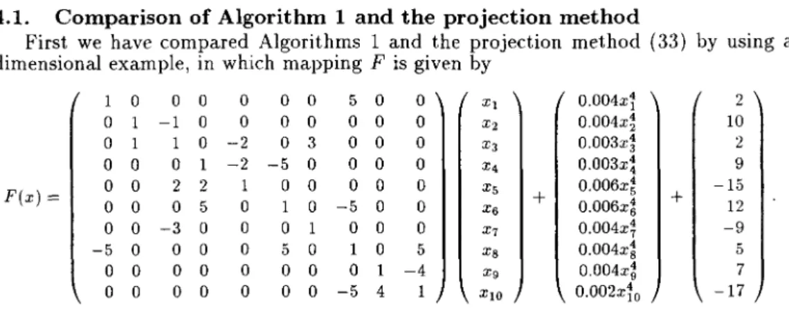
First we have compared Algorithms 1 and the projection method (33) by using a 10-dimensional example, in which mapping F is given by

1 0 0 0 0 0 0 5 0 0 Xl 0.004xi 2 0 -1 0 0 0 0 0 0 0 X2 0.004x~ 10 0 1 1 0 -2 0 3 0 0 0 X3 0.003x~ 2 0 0 0 -2 -5 0 0 0 0 X4 0.003x! 9 F(x) == _{0 0}0 0 _{0 5}2 2 ₀ 0 0 _{1 0} _{-5 0}0 0 0 ₀ Xs _X6

+

0.006x~ _0.006xt

+

-15 ₁₂ 0 0 -3 0 0 0 0 0 0 X7 0. 004X

f

-9 -5 0 0 0 0 5 0 1 0 5 Xs 0.004x~ 5 0 0 0 0 0 0 0 0 1 -4 Xg 0.004x~ 7 0 0 0 0 0 0 0 -5 4 XIO 0.002xio -17

The results for this problem are shown in Table 1.

In general, the projection method is guaranteed to converge, only if the parameter b

is chosen sufficiently large. In fact, Table 1 shows that when {j is large, the projection met.hod is always convergent, but as {j becomes small, the behavior of the method found to

be unstable and eventually it fails to converge.

Table 1 also shows that Algorithm 1 is always convergent even if {j is chosen small, since

the line search determines an adequate step size at each iteration. In Algorithm 1, the number of iterations is almost constant. This is because we may choose a larger step size when the magnitude of vector dk _{is small, i.e. b is large.}

Algorithm 1 spends more CPU times per iteration than the projection method, because the former algorithm requires overheads of evaluating the merit function

f.

But, when b

becomes large, Algorithm 1 tends to spend less CPU time than the projection method, because the number of iterations of Algorithm 1 increases mildly.

4.2. Comparison of Algorithm 2 and Newton method

Next we have compared Algorithm 2 and the pure Newton method (18) without line search. For each of the problem sizes n = 30,50 and 90, we randomly generated five test problems. The parameters p and {j were set as p = 1 and {j = 1. The starting point was chosen to be x = O. In solving the linearized subproblem at each iteration of Algorithm 2 and Newton method, we used Lemke's complementarity pivoting method [13] coded by Fukushima [11]. All parameters and starting points are set to the default values used in [11]. The results are given in Table 2. All numbers shown in Table 2 are averages of the results for five problems for each case and #Lemke is the total number of pivotings in Lemke's method.

Table 2: Comparison of Algorithm 2 and Newton method

(p

= 1).

Algorithm 2 Newton method

n #Iterations

_#f

#Lemke CPU #Iterations #Lemke CPU

30 5.6 7.6 80.6 4.294 8 115.2 !i.840

50 5.6 7.Ei 156.0 19.880 8 216.4 26.142

90 6.0 8.0 275.2 105.400 8 358.8 135.690

Table 2 shows that the number of iterations of Newton method is consistently larger than that of Algorithm 2 as far as the test problems used in the experiments are concerned. Therefore, since it is time consuming to solve a linear sub problem at each iterat.ion, Algo-rithm 2 required less CPU time than the pure Newton method in spit.e of the overheads in line search. Finally we note that, the pure Newton method (18) is not guaranteed to be

(16)

globally convergent, although it actually converged for all test problems reported in Table 2.

4.3. Comparison of Algorithms 1 and 2

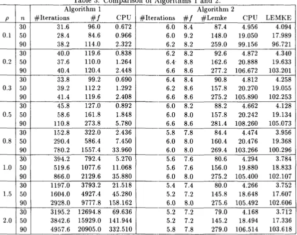
Finally we have compared Algorithms 1 and 2. For each of the problem sizes n

=

30,.50 and 90, we randomly generated five test problems. To see how these algorithms behave for various degrees of asymmetry of the mapping F, we have tested several va.lues of p between 0.1 and 2.0. The starting point was chosen to be x = O. The results are given in Table 3. All numbers shown in Table 3 are averages of the results for five test problems for each case.

Table 3: Comparison of Algorithms 1 and 2.

Algorithm 1 Algorithm 2

p n #lterations

_#f

CPU

#lterations

_#f

#Lemke

CPU

LEMKE

30 :n.6 96.0 0.672 6.0 8.4 87.4 4.9156 4.094 0.1 50 28.4 84.6 0.966 6.0 9.2 148.0 19.050 17.989 90 3.8.2 114.0 2.322 6.2 8.2 259.0 99.156 96.721 30 40.0 119.6 0.838 6.2 8.2 92.6 4.872 4.340 0.2 50 3:7.6 110.0 1.264 6.4- 8.8 162.6 20.888 19.633 90 40.4 120.4 2.448 6.6 8.6 277.2 106.672 103.201 30 3:3.8 99.2 0.690 6.4 8.4 90.8 4.812 4.258 0.3 50 3:9.2 112.2 1.292 6.2 8.6 157.8 20.270 19.055 90 41.4 119.6 2.408 6.6 8.6 275.2 105.890 102.253 30 45.8 127.0 0.892 6.0 8.2 88.2 4.662 4.128 0.5 50 E,8.6 161.8 1.848 6.0 8.0 157.8 20.242 19.134 90 110.8 273.8 5.780 6.6 8.6 281.4 108.260 105.073 30 1E,2.8 322.0 2.436 5.8 7.8 84.4 4.474 3.956 0.8 50 2£10.4 586.4 7.450 6.0 8.0 160.4 20.476 19.368 90 780.2 1557.4 33.960 6.0 8.0 269.4 103.266 100.296 30 394.2 792.4 5.270 5.6 7.6 80.6 4.294 3.784 1.0 50 519.6 1077.6 11.068 5.6 7.6 156.0 19.880 18.833 90 8(;6.0 2129.6 35.880 6.0 8.0 275.2 105.400 102.107 30 1Hi7.0 3793.2 21.518 5.4 7.4 80.0 4.266 3.752 1.5 50 1604.0 4927.4 45.280 5.2 7.2 145.8 18.648 17.607 90 2928.0 9777.8 158.162 6.0 8.0 275.6 105.492 102.606 30 3Hi5.2 12694.8 69.636 5.2 7.2 79.0 4.168 3.712 2.0 50 3842.6 15929.0 141.944 5.2 7.2 145.2 18.494 17.336 90 49ii7.6 20905.0 332.510 5.8 7.8 279.0 106.514 103.618 Table 3 shows that when the mapping F is close to symmetry, Algorithm 1 converges very

fast, and when the mapping becomes asymmetric, the number of iterations and CPU time of Algorithm 1 increase rapidly. On the other hand, in Algorithm 2, while the total number of pivotings of Lemke's method increases in proportion to problem size n, the number of iterations stays constant even when the problem size and the degree of asymmetry of Fare varied. Hence, when the degree of asymmetry of F is relatively small, that is, when p is smaller than 1.0 in our test problems, Algorithm 1 requires less CPU time than Algorithm 2.

Note that, since the mapping F used in our computational experience is sparse, com-plexity of each iteration in Algorithm 1 is small. On the other hand, the code [11] of Lemke's method used in Algorithm 2 to solve a linear subproblem does not make use of sparsity.

(17)

Moreover, since Lemke's method is restrictive in the choice of initial points, at each iteration we must restart from a priori fixed initial point even when the iterate becomes close to a solution. Therefore, it may require a significant amount of CPU time at each iteration for large problems. (In Table 3, LEMKE is the total CPU time to solve subproblems by Lemke's method.) If a method that can make use of sparsity and can start from arbitrary point is available to solve a linear subproblem, CPU time of Algorithm 2 may decrease. (For the latter respect, the path-following method of van der Laan and Talman [19] might be useful.) The projected Gauss-Seidel method [3, pp. 397] for solving linear complementarity problem is one of such methods. In Table 4, results of Algorithm 2 using the projected Gauss-Seidel method in place of Lemke's method are given. Table 4 shows that, if the mapping F is almost symmetric, Algorithm 2 converges very fast. But Algorithm 2 fails to converge when the degree of asymmetry increased, because the projected Gauss-Seidel method failed to solve linear subproblems.

() ()

«

Table 4: Results for Algorithm 2 (Gauss-Seidel version).

p n 30 0.1 50 90 30 0.2 50 90 30 0.3 '" 2.0 50 90 10 \::,'," .... "l. 0.1 0.01 0.001 0.0001 1e-05 1e-06 0 2 Algorithm 2

#Iterations

_#f

#Gauss CPU

6.0 8.4 39.2 0.274 6.0 9.2 39.6 0.466 6.2 8.2 48.0 0.916 3 of 5 failed 3 of 5 failed failed failed . ... · · · · K

~g:g:~ ~

:=

4 ... ... n=30:Algorithm 20 11\50:Algorithm 2x 6 8 10

CPU time (sec.)

... ~"

12

""

14 Figure 1: Behavior of Algorithms 1 and 2.

(18)

Figure 1 illustrates how Algorithms 1 and 2 converged for two typical test problems with

n = 30 and 50. In the figure, the vertical axis represents the accuracy of a generated point to the solution, which is evaluated by

ACC

=

max

{I

min(xi, Fi(;r))11 i

=

1,2, ... , n}.

I

Figure 1 indicates that Algorithm 2 is quadratically convergent near the solution. Figure 1 also indicates that Algorithm 1 is linearly convergent though it has not been proved theoretically.

5. Computational results 11

In this section, we present the results of applying Algorithms 1 and 2 to some examples which arise from an optimization problem, a spatial price equilibrium problem, a nonco-operative game and a traffic assignment problem. The algorithms were implemented in FORTRAN on a SUN-4 workstation. The parameters in the algorithms were set in the same manner as in Section 4. The positive diagonal matrix D was also chosen to be the identity matrix multiplied by {j

>

0, and hence the merit function (32) was used. The convergence criterion was

I

min(xi, Fi(X))1 :::; CC for all i

=

1,2, ... , n,

where CC is a parameter used to change accuracy of algorithms. In solving the linearized subproblem of Algorithm 2, we used Lemke's complementarity pivoting algorithm coded by Fukushima [11]. The results are shown in Tables 5 '" 11.

Some mappings used in the experiments were only monotone but not strongly monotone. Others were not even monotone, though they could be considered almost monotone. Thus all the problems do not satisfy the convergence conditions of our algorithms. However, for the most case both Algorithms 1 and 2 converged and produced satisfactory solutions. Example 1 This is the following 4-variable complementarity problem from Josephy [12], whose mapping is given by

(

3xi

+

2XIX2

+

2x~

+

X3

+

3X4 - 6 )

F( ) _

2xi

+

Xl

+

x~

+

3X3

+

2X4 - 2 X - 3xi

+

XIX2

+

2:r~

+

2X3

+

3X4 - 1 .

xi

+

3x~

+

2X3

+

3X4 - 3

The results are shown in Table 5. Since the mapping is co-positive but not monotone, Algorithm 2 failed when the initial points (0, ... ,0) and (10, ... , 10) were chosen, because the linearized subproblem at (0, ... ,0) has no solution and the search direction at (10, ... ,10) is not a descent direction, respectively. On the other hand, Algorithm 1 converged for those initial points.

Table 5: Results of Example 1.

CC Initial point #Iterations

_#f

CPU #Iterations

_#f

#Lemke CPU

10-5 _{(0, ... ,0)} ₂₀ ₆₂ _0.00 _failed

(1, ... ,1) 21 63 0.00 4 5 8 0.00

(5, ... ,5) 21 63 0.00 5 6 10 0.00

(19)

Example 2 This is a 10-variable complementarity problem arising from the Nash-Cournot production problem appeared in Harker [9]. In this example, the Jacobian \;' F(x) of the mapping is a P-matrix for any x

>

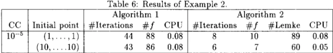
0, but the mapping F is not monotone. Table 6 shows that both Algorithms 1 and 2 converged to the solution quickly.

_#f

CPU #Iterations

#f

#Lemke

10-5 _{(1, ... , 1)} ₄₄ ₈₈ _0.08 ₈ ₁₀ ₈₉

(10, .... 10) 43 86 0.08 6 7 60

Example 3 This example is the following convex programming problem: mInImIZe CrI - 10)2

+

5(X2 - 12)2

+

x~

+

3(X4 - 11)2

+

10x~ +7x~

+

2x~ - 4X6X7 - 10x6 - 8X7 subject to 2xi

+

3x~

+

X3

+

4x~

+

5x§ ::; 100 7XI

+

3X2

+

10x~

+

X4 - X5 ::; 200 20Xl

+

x~

+

6x~ - 8X7 ::; 150 4xi

+

x~ - 3XIX2

+

2x~

+

5X6 - 11X7 ::; 0 Xi ;::: 0, i = 1,2, ... ,7, CPU 0.08 0.05

which is formulated as an 11-variable complementarity problem. Since the objective function is convex, the mapping is monotone, but not strongly monotone on R~. Table 7 shows that Algorithms 1 and 2 converged for both initial points (0, ... ,0) and (10, ... ,10).

Table 7: Results of Example 3

CC Initial point #lterations

_#f

CPU #Iterations

_#f

#Lemke CPU

10 3 (0, ... ,0) 263 840 0.13 5 10 :~O 0.03

(10, .... 10) 1213 4504 0.64 9 10 '75 0.08

10 5 _{(0, ... ,0)} ₃₇₅ ₁₁₁₉ _0.19 ₆ ₁₁ _:~6 _0.04

(10, .... 10) 1308 4752 0.67 10 11 81 0.08

Example 4 This example is a 15-variable traffic assignment problem from Bertsekas and Gafni [2]. This problem consists of a traffic network with 25 nodes, 40 arcs, 5 O-D pairs and 10 paths. The mapping is monotone but not strongly monotone. The ('esults are shown in Table 8. In this example, Algorithm 1 failed to find a descent direction because the mapping is not strongly monotone. But Algorithm 2 converged in 4 iterations for both initial points.

_#f

CPU #Iterations

_#f

#Lemke CPU

10 3 _{(0, ... ,0)} ₁₇₁₈₁ _failed ₄ _.5 ₆₂ _0.09

(1, .... 1) 16608 failed 4 5 64 0.10

10 5 _{(0, ... ,0)} ₁₇₁₈₁ _failed ₄ ₅ ₆₂ _0.09

(20)

Example 5 This example is the following convex programming problem:

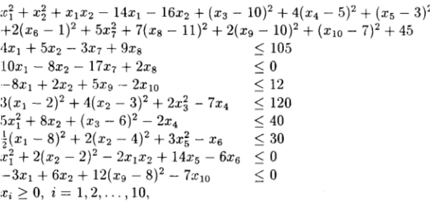
mImmIze :ct

+

X~

+

XIX2 - 14XI - 16x2

+

(X3 - 10)2

+

4(X4 - 5)2

+

(X5 - 3)2

+2(X6 - 1)2

+

5x~

+

7(xg - 11)2

+

2(xg - 10)2

+

(XlO - 7)2

+

45 subject to 4XI

+

5X2 - 3X7

+

9xg ::; 105 lOXI - 8X2 - 17x7

+

2xg ::; 0 -8XI

+

2X2

+

5xg - 2XlO :~(XI - 2)2

+

4(X2 - 3)2

+

2x~ - 7X4 Sxi

+

8X2

+

(X3 - 6)2 - 2X4 ~(XI - 8)2

+

2(X2 - 4)2

+

3x~ - X6

:ri

+

2(xz - 2)2 - 2xrxz

+

14x5 - 6X6 -3XI

+

6X2

+

12(xg - 8)2 - 7:ClO ;ri ~ 0, i = 1,2, ... , 10, ::; 12 ::; 120 ::; 40 ::; 30

::;0

which is formulated as an 18-variable complementarity problem. The results are shown in Table 9. The mapping is monotone but not strongly monotone. Algorithm 1 converged slowly and eventually failed to find a descent direction as the iterate become very close to a solution. On the other hand, Algorithm 2 converged in several iterations for both initial points.

CC

Initial point #Iterations

_#1

CPU

#Iterations

_#1

#Lemke

CPU

10-

3 _{(0, .... 0)}

31616 414381 71.98 4 5 68 0.14 (10, .... 10) 31238 411704 72.43 6 7 97 0.19

10

5 _{(0, .... 0)} ₇₂₀₅₀ _failed ₅ ₆ ₈₄ _0.17

(10, .... 10) 75257 failed 6 7 97 0.19 Example 6 This example is a spatial price equilibrium problem from Tobin [18] which is formulated as a 42-variable complementarity problem. The mapping is not monotone but is close to be monotone. The results are shown in Table 10.

CC

Initial point #Iterations

_#1

CPU

#lterations

_#1

#Lemke

CPU

10

-3 _{(0, ... ,0)} ₆₃ ₁₄₈ _0.09 ₆ ₁₁ ₁₃₀ _1.34 (1,. ., 1) 66 155 0.09 7 10 131 1.37 (10, .... 10) 63 149 0.10 7 8 157 HiD 10 5 _{(0, ... ,0)} ₈₄ ₁₉₉ _0.12 ₇ ₁₂ ₁₄₈ _Ui3 (1, ... ,1) 89 209 0.12 7 10 131 UI7 (10, .... 10) 83 197 0.12 7 8 157 1.(;0 In this example, Algorithms 1 and 2 converged for all initial points chosen in our experiment. Note that the mapping of Example 6 is similar to the form (34) used in the experiments of Section 4, and hence, the mapping is sparse. For the example, Algorithm 1 converged mush faster than Algorithm 2.

Example 7 This example is a traffic assignment problem. This is a 40-variable comple-mentarity problem which is Example 6.2 in Aashtiani [1]. The results are shown in Table 11. The mapping is monotone but not strongly monotone. For this example, Algorithm 1 converged slowly and could not attain the strict convergence criterion

CC= 10-

5

(21)

other hand, Algorithm 2 failed because the linear subproblem became unsolvable after 2 or 3 iterations.

_#f

CPU #Iterations

#f

#Lemke CPU

10 3 _{(0, ... ,0)} _{2907 24925} _13.25 ₂ _failed

(10, .... 10) 2981 25797 13.74 3 failed

10 5 (0, ... ,0) 4218 failed 2 failed

(10, .... 10) 4166 failed 3 failed

6. Concluding remarks

When the mapping is strongly monotone with modulus /1, the solution x* to (1) satisfies the inequality

II

x*

11::::

~

II

F(O)

II .

/1

Hence, we may reform problem (1) as a variational inequality with bounded constraint by adding an extra constraint

II

x

1100:::: R

with a sufficiently large positive number R, and apply the methods of Fukushima [7] or Taji et al. [17] directly. Then the subproblem becomes a linear variational inequality problem with a bound constraint, which is in general more difficult to solve than a linear complementarity problem of the proposed algorithms.

Since the modulus /1 is generally a priori unknown, if the matrix D is chosen not to satisfy

liD II

<

4/1, Algorithm 2 may fail because the search direction is not guaranteed to be a descent direction. When we do not know the exact value of /1 for the strongly monotone mapping F, we may start Algorithm 2 with a suitable value of /1, and, if it fails, continue by halving D until convergence is obtained. Eventually we will have

II

D

II

<

4/1 and hence Algorithm 2 must converge by Theorem 2.

Acknowledgement The authors are grateful to Professor T. Ibaraki of Kyoto University and the refrees for helpful comments.

References

[1] Aashtiani, H. Z.: The Multi-modal Traffic Assignment Problem. Ph. D. thesis, Sloan School of Management, Massachusetts Institute of Technology, Cambridge, MA, 1979. [2] Bertsekas, D. P. and Gafni, E. M. : Projection Methods for Variational Inequalities with Application to the Traffic Assignment Problem, Mathematical Programming Study, vol. 17 (1982), 139-159.

[3] Cottle, R. W., Pang, J. S. and Stone, R. E.: The Linear Complementarity Problem, Academic Press, San Diego, 1992.

[4] Dafermos, S.: Traffic Equilibrium and Variational Inequalities. Transportation Science, vol. 14 (1980), 42-54.

[5] Dennis, J. E. and Schnabel, R. B.: Numerical Methods for Unconstrained Optimization and Nonlinear Equations, Prentice-Hall, Eaglewood Cliffs NJ, 1983.

[6] Florian, M.: Mathematical Programming Applications in National, Regional and Urban Planning. Mathematical Programming: Recent Developments and Applications, Iri, M. and Tanabe, K. (eds.), KTK Scientific Publishers, Tokyo, 1989.

(22)

[7] Fukushima, M.: Equivalent Different.iable Optimization Problems and Descent Meth-ods for Asymmetric Variational Inequality Problems. Mathematical Programming, vol. .53 (1992), 99-110.

[8] Garcia, C. B . .and Zangwill, W. I.: Pathways to Solutions, Fixed Points, and Equilibria Prentice-Hall, Eaglewood Cliffs NJ, 1981.

[9] Harker, P. T.: Accelerating the Convergence of the Diagonalization and Projection Al-gorithms for Finite-Dimensional Variational Inequalities. Mathematical Programming, vol. 41 (1988). 29-59.

[10] Harker, P. T. and Pang, J. S.: Finite-Dimensional Variational Inequality and Nonlin-ear Complementarity Problems: A Survey of Theory, Algorithms and Applications. Mathematical Programming, vol. 48 (1990),-161-220.

[11] Ibaraki, T. and Fukushima, M.: FORTRAN 77 Optimization Programming (in Japa.nese), Iwanami-Shoten, Tokyo, 1991.

[12] Josephy, N. H.: Newton's Method for Generalized Equations. Technical Report No. 1965, Mathematics Research Center, University of Wisconsin, Madison, WI, 1979 [13] Lemke, C. E.: Bimatrix Equilibrium Points and Mathematical Programming.

Manage-ment Science, vol. 11 (1965),681-689.

[14] Marcotte, P . .:l,nd Dussault, J. P.: A Sequential Linear Programming Algorithm for Solving Monotone Variational Inequalities. SIAM Journal on Control and Optimization, vol. 27 (1989), 1260-1278.

[15] Mathiesen, L.: An Algorithm Based on a Sequence of Linear Complementarity Prob-lems Applied to a Walrasian Equilibrium Model: An Example. Mathematical Program-ming, vo!. 37 1)987), 1-18.

[16] Pang, J. S. and Chan, D.: Iterative Methods for Variational and Complementarity Problems. Mathematical Programming, vol. 24 (1982), 284-313.

[17] Taji, K., Fukushima, M. and Ibaraki, T.: A Globally Convergent Newton Method for Solving Strongly Monotone Variational Inequalities. Mathematical Programming, vol. 58 (1993), 369-383.

[18] Tobin, R. L.: A Variable Dimension Solution Approach for the General Spatial Price Equilibrium Problem. Mathematical Programming, vo!. 40 (1988), 33-51.

[19] Van der Laan, G. and Talman, A. J. J.: An Algorithm for the Linear Complemen-tarity Problem with Upper and Lower Bounds. Journal of Optimization Theory and Applications, vo!. 62 (1989), 151-163.

Kouichi TAJI and Masao FUKUSHIMA: Graduate School of Information Science,

Advanced Institute of Science and Technology, Nara, Takayama, Ikoma, Nara 630-01, Japan