Strict and Strong Quasi-Concavity：What is the Difference ?

Strict and Strong Quasi-Concavity：What is the

Difference ?

著者

Koide Hiroyuki

journal or

publication title

THE NAGOYA GAKUIN DAIGAKU RONSHU; Journal of

Nagoya Gakuin University; SOCIAL SCIENCES

volume

46

number

3

page range

1-12

year

2010-01-31

　 Frequent appearance of quasi-concave functions in microeconomic theory is the proof of their importance, and yet they can be a stumbling block to the rigorous and deep understanding of the theory. This may be partly attributed to so many concavity-related concepts and various characterizations.1)

In particular, strict quasi-concavity and strong quasi-concavity are sometimes confused and treated equivalently. This paper aims to explore the subtle relations among concavity, strict quasi-concavity and strong quasi-quasi-concavity in a unified manner.

1. Basic facts

　 Let f（x） be a real-valued function defined on a convex subset S of Rn _{and x ＝（x}

1， x2， …， xn）′ be a

point in S.2)

Definition 1　f（x） is quasi-concave on S if for all x1 _{and x}2_{∈S and all α∈［0, 1］}

f（αx1_{＋（1－α）x}2_{）≧min｛ f（x}1_），f（x2_{）｝ (1)} Definition 2　f（x） is strictly quasi-concave on S if for all x1_≠x2_∈S3) _{and all α∈［0, 1］}

f（αx1_{＋（1－α）x}2_{）＞min｛ f（x}1_），f（x2_{）｝ (2)}

　 When f（x） is a twice-continuously differentiable function, quasi-concavity can be characterized in terms of the leading principal minors of the bordered Hessian matrix. Let

D（r x）≡ 0 f（1 x） f2（x） …… f（r x） f（1 x） f11（x） f12（x） …… f1r（x） f（2 x） f21（x） f22（x） …… f2r（x） … … … … fr （x） fr1（x） fr2（x） …… frr（x） where4) fi （x）≡∂_∂f（x）_x i ，i＝1，2，… r，

Strict and Strong Quasi-Concavity：What is the Difference ?

Hiroyuki Koide

f（ij x）≡

∂2f（x）

∂xi∂xi，i， j＝1， 2，… r．

Theorem 1　If f（x） is a quasi-concave function of class C2 _{defined on an open convex set S, then}

（－1）r _D r

（x）≧0，r＝2，3，…，n，for all x∈S. (3)

(Proof) See Arrow and Enthoven (1961) or Kemp and Kimura (1978).

　 Needless to say, condition (3) is trivially satisfied for r＝1. As for sufficiency, Arrow and Enthoven (1961) showed that condition (14) below is sufficient for quasi-concavity, which, in fact, is strong enough to guarantee strict quasi-concavity and more. Before proving this, we give a brief review of quadratic forms, which is essential to the subsequent analysis.

2. Definite and semidefinite quadratic forms

　 Consider a quadratic form

Σ

Σ

b11h1＋b12h2＋…＋b1nhn＝0，

b21h1＋b22h2＋…＋b2nhn＝0，

… (5) bm1h1＋bm2h2＋…＋bmnhn＝0，

where we assume m＜n and

b11 b12 …… b1m

b21 b22 …… b2m

… … …

bm1 bm2 …… bmm

≠0. (6)

For the sake of simplicity (4) ～ (6) are rewritten in matrix forms:5) h′A h,

B h＝0, ｜Bmm｜≠0,

where A＝（aij）, B＝（bij）, h＝（h1， h2，…， hn）′, and Bkl is the matrix formed by the first k rows and the first l columns of B. The associated determinants with this quadratic form are expressed as

Hr≡ 0 Bmr （Bmr）′ Arr

＝ 0 …… 0 b11 …… b1r … … … … 0 …… 0 bm1 …… bmr b11 …… bm1 a11 …… a1r … … … … b1r …… bmr ar1 …… arr ，r＝1，2，…，n． (7)

Furthermore, let π denotes a permutation of ｛1, 2, …, n ｝ and Aπ

denote the matrix obtained from A after performing the permutation π on its rows and columns. Similarly, let Bπ

denote the matrix obtained from B after performing the permutation π on its columns. Thus, for example, Aπ

rr is the matrix formed by the first r rows and the first r columns of Aπ

. Bπ

mr is similarly interpreted. When with permutation π , determinants (7) are rewritten as

H ~ r≡ 0 Bπ mr （Bπ mr）′ Aπrr ，r＝1，2，…，n． Theorem 2　Let ｜Bmm｜≠0.

(1) h′A h＜0 for all h∈｛h∈Rn_{｜B h＝0，h≠0｝ if and only if} （－1）r _H

r＞0，r＝m＋1，…， n， (8)

(2) h′A h≦0 for all h∈｛h∈Rn_{｜B h＝0｝ if and only if} （－1）r _H~

r≧0，r＝m＋1，…，n，for all π. (9)

(Proof) See Debreu (1952).6)

　 The relation between negative definiteness and negative semidefiniteness (that is, when a negative semidefinite matrix becomes negative definite) is given by the following theorem, which is rarely seen in the economic literature.7)

Theorem 3　Let ｜Bmm｜≠0 and h′A h≦0 for all h∈｛h∈Rn｜B h＝0｝. Then h′A h＜0 for all h∈｛h∈

Rn_{｜B h＝0，h≠0｝ if and only if}

Hn＝

0 B

B′ A≠0. (10)

(Proof) Sufficiency Suppose h′A h＝0 for some h≠0. Then since such h attains a maximum of the quadratic form under the linear constraints which are linearly independent, there exist a set of multipliers, λ＝（λ1，λ2，…，λm）′, such that

2A h＋B′λ＝0

These equations can be rewritten in a matrix form as 0 B B′ A （1/2）λ h ＝0, (11)

which, in consideration of h≠0, implies that the coefficient matrix of (11) is singular. This contradicts the assumption of (10).

Necessity Suppose the determinant (10) is zero. Then there exist vectors h∈Rn _{and λ∈R}m _{such that} （h′，λ′）≠0′ and 0 B B′ A λ h ＝0, that is, B h＝0 (12) B′λ＋A h＝0. (13)

If h＝0, then B′λ＝0, which implies λ＝0 since the linear constraints are independent by the

assumption that ｜Bmm｜≠0. Therefore, h≠0. From (12) and (13) we have

h′A h＝－h′B′λ＝0

This contradicts the assumption that A is negative definite under the condition B h＝0. Q. E. D. Now, we are ready to prove the following theorem.

Theorem 4　Let f（x） be a function of class C2 _{defined on an open convex set S. If}

（－1）r _D r

（x）＞0，r＝1，2，…，n，for all x∈S, (14)

then f（x） is strictly quasi-concave on S.

(Proof) Since it is already proved by Arrow and Enthoven (1961) that (14) is sufficient for f（x） to be concave, we have only to induce contradiction by assuming that f（x） is not strictly quasi-concave. Suppose f（x） is quasi-concave but not in the strict sense. We can find two distinct points x1

and x2∈S （let f（x1）≧f（x2）） such that there exists α˜∈（0，1） for which

F（α˜）≡f（α˜x1＋（1－α˜）x2）＝f（x2） (15)

and

As can be seen from Figure 1, α˜ achieves a minimum. Hence we have the following conditions: dF（α˜） dα ＝∇f（α˜x1＋（1－α˜）x2）（x1－x2）＝0 (16) and d2_F（α˜） dα2 ＝（x1－x2）′∇2f（α˜x1＋（1－α˜）x2）（x1－x2）≧0, (17) where ∇f（x）≡（ f（1 x）， f2（x），…， f（n x）） and ∇2f（x）≡ f11（x） f12（x） …… f1n（x） f21（x） f22（x） …… f2n（x） … … … fn1（x） fn2（x） …… fnn（x） .

Note that the assumption of f（1 x）≠0 is concealed in (14). Then according to Theorem 2, condition (14)

implies that the quadratic form in (17) must be negative subject to the linear constraint (16). This is a

contradiction. Q. E. D.

3. Katzner’s example

　 It is important to note that the converse of Theorem 4 does not necessarily hold. In other words, even if we limit f（x） to be strictly quasi-concave in Theorem 1, we cannot delete equality from condition (3). Although this is a case of a strictly concave function, it may be of some help for the understanding of this point to cite an example of y＝－x4_{. In this case, y is strictly concave in x, but}

d2_y/dx2_{＜0 does not hold at x＝0. With this in mind, it is recognized that an indifference curve y＝y（x，u）}

derived from a strictly quasi-concave function u＝f（x，y） is indeed strictly convex in x and nevertheless d2_y/dx2_{＝0 may happen on a nowhere dense subset of R. A good example given by Katzner (1970) is}

examined below. 8)

　 Consider the utility function defined on the positive orthant by

f（x，y）＝x3_y＋xy3_{. (18)}

An indifference curve for (18) is given by x3_y＋xy3_＝a

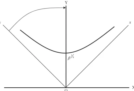
for a certain constant a＞0. To grasp a clear image of this curve, we rotate the axis x―O―y by （－45°） and express the new one by X―O―Y. Then using the rotation formula

x＝X cos（－45°）－Y sin（－45°） and

y＝X sin（－45°）＋ Y cos（－45°）, we obtain

Y4_＝X4_＋β,

where β＝2a. As can be seen from Figure 2, the indifference curve Y＝（X4_＋β）1/4 _{is strictly convex in}

X, and hence (18) is a strictly quasi-concave function. The bordered Hessian can be easily calculated as D（2 x）≡ 　 0 y（3x2_＋y2_{） x（x}2_＋3y2_） y（3x2_＋y2_{） 　 6xy 3（x}2_＋y2_） x（x2_＋3y2_{） 3（x}2_＋y2_{） 　 6xy} .

Hence D（2 x） calculated along the line y＝x is zero, which corresponds to the fact that d2Y/dX2＝0 along

the Y-axis in the new coordinate system.

　 The geometrical meaning of nonvanishing Bordered Hessian is clarified in terms of curvature of a curve. Curvature is a measure of the rapidity with which curves change directions.9) _{When a curve is}

given in the form y＝f（x）, its curvature κ at （x, y） is calculated as κ≡ f ″（x）

1＋（ f ′（x））32 .

If f ″（x）＝0, the curvature is also zero, which is exactly the case with Katzner’s example. Obviously nonzero curvature implies that the marginal rate substitution between any two goods is strictly diminishing.

4. Strong quasi-concavity

　 To avoid the possibility of D（r x）＝0 for a strictly quasi-concave function, we need a stronger concept of quasi-concavity than that of strict quasi-concavity à la Barten and Böhm (1982).10)

Definition 3　Let f（x） be a function of C2 _{class defined on an open convex set S. f（x） is strongly}

quasi-concave if11)

h′∇2_{f（x）h＜0 for all x∈S and h∈｛h∈R}n_{｜∇f（x）h＝0，h≠0｝. (19)}

　 As can be expected from the definition, strong quasi-concavity implies strict quasi-concavity.

Theorem 5　Let f（x） be a function of class C2 _{defined on an open convex set S. If f（x） is strongly}

quasi-concave, then f（x） is strictly quasi-concave as well.

(Proof) Suppose f（x） is not strictly quasi-concave. Then we can find two distinct points x1 and x2∈S

（let f（x1）≧f（x2）） such that there exists α′∈（0，1） for which

F（α′）≦F（0）,

where F（α） is defined by (15). If F（α′）＜F（0）, there must exist α˜∈（0，1） such that F（α˜） is a minimum. If F（α）≧F（0） for all α∈［0, 1］, F（α′） is also a minimum. Thus in either case, there exists α˜∈（0，1） which achieves a minimum of F（α）. This requires conditions (16) and (17), which

contradicts (19). Q. E. D.

　 Now letting A＝∇2_f（x0_{） and B＝∇f（x}0_{） in Theorem 2 and Theorem 3, we know that}

quasi-concavity of f（x） is closely related to negative definiteness (or semidefiniteness) of the quadratic form determined by its Hessian matrix under the linear condition which is also related to the hyperplane tangent to the level set ｛x∈Rn_{｜f（x）≧ f（x}0_）｝.12) _{Such relation can be compactly summarized by the}

following theorem.

Theorem 6　Let f（x） be a function of class C2 _{defined on an open convex set S and ∇f（x）≠0 for all} x∈S. Then f（x） is quasi-concave if and only if

h′∇2f（x）h≦0 for all x∈S and h∈｛h∈Rn_{｜∇f（x）h＝0｝. (20)}

(Proof) See Otani (1983).

　 In this theorem, the condition “∇f（x）≠0 for all x∈S” cannot be dropped, in particular, for the sufficiency part.13） _{For example, consider a strictly convex function y＝x}4_{. Since condition (20) is}

trivially satisfied by x＝0, we check this condition for x≠0. Then ∇f（x）h＝0 holds only at h＝0, where h′∇2_{f（x）h≦0 is satisfied. But this does not imply that y＝x}4 _{is quasi-concave.}

From Definition 3 and Theorem 2, we obtain the following theorem.

Theorem 7　Let f（x） be a function of class C2 _{defined on an open convex set S and f} 1

（x）≠0 for all x∈S. Then f（x） is strongly quasi-concave if and only if

（－1）r _D r

（x）＞0，r＝2，3，…，n，for all x∈S. (21)

　 Since the condition f（1 x）≠0 can be squeezed into (21), condition (14) in Theorem 4 is, in fact,

strong enough to imply strong quasi-concavity of f（x）.

　 The following theorem is a generalized version of Theorem 11.2 of Barten and Böhm (1982), but our proof is much simpler.

Theorem 8　Let f（x） be a quasi-concave function of class C2 _{defined on an open convex set S and}

∇f（x）≠0 for all x∈S. Then f（x） is strongly quasi-concave if and only if

D（n x）≠0 for all x∈S. (22)

(Proof) Sufficiency If f（1 x）≠0 for all x∈S, then by Theorem 6 quasi-concavity of f（x） is equivalent

to condition (20), which, in consideration of Theorem 3 and condition (22), is equivalent to (19). If f（1 x）＝0 for some x∈S, we have f（i x）≠0 for at least one i∈｛2，3，…，n｝ since ∇f（x）≠0 for all x∈ S. Hence we can choose an appropriate permutation π (i.e. renumbering of variables) so that the first element of （∇f（x））π

h′（∇2_{f（x））h≦0 for all x∈S and h∈｛h∈R}n_{｜（∇f（x））h＝0｝,} and this implies

h′（∇2_f（x））π_{h＜0 for all x∈S and h∈｛h∈R}n_{｜（∇f（x））}π_{h＝0，h≠0｝,}

if the associated bordered Hessian matrix is nonsingular. Since permutation π does not change the value of the bordered Hessian determinant, condition (22) is sufficient to imply strong quasi-concavity of f（x）.

Necessity Since ∇f（x）≠0 for all x ∈ S, quasi-concavity of f（x） implies condition （20） by Theorem 6. We can safely assume f（1 x）≠ 0 for all x ∈ S with renumbering of variables, if necessary, as we did

above. Hence strong quasi-concavity of f（x） implies condition （22） by Theorem 3. Q. E. D. 　 In fact, we can omit the regularity condition “∇f（x）≠0 for all x ∈ S” when applying the sufficiency part of Theorem 8, for condition （22） itself implies this condition. Similarly, we can also omit the regularity condition “f（1 x）≠0 for all x ∈ S” when applying the sufficiency part of Theorem 3 to relate

condition （20） to condition （19）, for condition （22） permit us to safely assume f（1 x）≠0 for all x ∈ S

with renumbering of variables, if necessary. 　 Finally, Theorem 1 can be generalized as follows.

Theorem 9　Let f（x） be a function of class C2 _{defined on an open convex set S and ∇f（x）≠0 for all} x∈S. Then f（x） is quasi-concave if and only if

（－1）r 　 0 （∇f（x））π r （（∇f（x））π r）′ （∇2f（x）） π rr

≧0，r＝2，3，…，n，for all x∈S and any π. (23)

(Proof) By Theorem 6, quasi-concavity of f（x） is equivalent to condition (20), which, in consideration of Theorem 2, is equivalent to condition (23). 14) _{Q. E. D.}

5. Conclusion

　 From the above theorems we can indicate the relations among various characterizations of quasi- concavity as in Figure 3.15) _{In this figure, an arrow should be read as “implies”and the determinant in}

(23) is denoted by Dπ

r （x）.

Figur

e 3

R

elations among V

Notes

1 ） For general discussion on quasi-concavity, see Diewert et al. (1981), Simon and Blume (1994) and Takayama (1994). 2 ） A dash (´) indicates transposition of vectors and matrices.

3 ） x1_≠x2_{∈S should be understood as x}1_{∈S, x}2_{∈S and x}1_≠x2_.

4 ） By the assumption that f（x） is of class C2_,

f（ij x）＝f（jix） for any i and j.

5 ） 0 stands for a vector or a matrix whose elements are all zeros. Needless to say, A is a symmetric matrix. 6 ） The necessary and sufficient conditions for A to be positive definite (positive semidefinite) are as follows:

（1） h′A h＞0 for all h∈｛h∈Rn_{｜B h＝0，h≠0｝ if and only if}

（－1）m_H

r＞0，r＝m＋1，…，n，

（2） h′A h≧0 for all h∈｛h∈Rn_{｜B h＝0｝ if and only if}

（－1）m~_H

r≧0，r＝m＋1，…，n，and for all π.

7 ） Theorem 3 is essentially the same as Theorem 9.4 of Hestenes (1966). 8 ） See Katzner (1970) p. 54.

9 ） See Protter (1988) p. 503.

10） See Barten and Böhm (1982), p. 405.

11） Incidentally, if ∇f（x）＝0, condition (19) implies strict concavity of f（x） in the neighborhood of x since its Hessian matrix is positive definite there.

12） This tangent hyperplane is expressed as

∇f（x0_）（x－x0_）＝0.

13）The regularity condition “ f（1 x）≠0 for all x∈S” is not used for the proof of the necessity part.

14） Since ∇f（x）≠0 for all x∈S, we can safely assume f（1 x）≠0 for all x∈S by renumbering the variables if necessary.

15） Figure 3 is supplemented with the following obvious relations: ① A strictly quasi-concave function is also quasi-concave. ② A positive definite quadratic form is also positive semidefinite.

References

Arrow, K. J. and A. C. Enthoven (1961), “Quasi-Concave Programming,” Econometrica, vol. 29, 779―800.

Barten, A. P. and V. Böhm (1982), “Consumer Theory,” in Arrow, K. J. and　M. D. Intriligator, eds., Handbook of Mathematical Economics, vol. 2, North-Holland, Amsterdam, 381―429.

Debreu, G. (1952), “Definite and Semidefinite Quadratic Forms,” Econometrica, vol. 20, 295―300.

Diewert, W. E., M. Avriel and I. Zang (1981), “Nine Kinds of Quasi-Concavity and Concavity,” Journal of Economic Theory, vol. 25, 397―420.

Hestenes, M. R. (1966), Calculus of Variations and Optimal Control Theory, Wiley, N. Y. Katzner D. W. (1970), Static Demand Theory, Macmillan, N. Y.

Kemp, M. C. and Y. Kimura (1978), Introduction to Mathematical Economics, Springer-Verlag, N. Y.

Otani, K. (1983), “A Characterization of Quasi-Concave Functions,” Journal of Economic Theory, vol. 31, 194―196. Protter, P. E. (1988), Calculus with Analytic Geometry, Jones and Bartlett Publishers, MA.

Simon C. and L. Blume (1994), Mathematics for Economists, Norton, N. Y.