B34
Ranking CMIP5 GCM Historical Runs for Optimum Model Ensemble Estimations over a
Regional Scale: A Case Study over Indochina Region
⃝ Rattana Chhin, and Shigeo Yoden
1. Introduction
Under the multimodel context, the awareness of limitation of the multiple model simulations through an evaluation study is very important before applying them to describe and understand the climate change. Rupp et al. (2013) described two primary goals motivating the evaluation of General Circulation Models (GCMs): (1) model developers’ evaluation efforts to identify model deficiencies and potential processes responsible for the deficiencies, and (2) evaluation for application which provides information about model uncertainty beyond that associated with climate projections. This study will focus on the second goal of climate model evaluation for impact assessment of climate change. We attempt to propose a framework of model evaluation and ensemble estimation for multiple perspectives of impact assessment (e.g., agriculture, water supply, hydropower, or flood control). We also aim at developing a routine to objectively select optimum ensemble members for climate change impact assessment over a specific region, by applying for Indochina region (ICR) as a case study.
2. Data and Method
This study uses APHRODITE as the observational dataset to evaluate GCMs. The APHRODITE dataset is recorded for the period of 1951-2007 with horizontal resolution of 0.25⁰ × 0.25⁰. We obtain the datasets for total 43 General Circulation Models (GCMs) to be evaluated over the case study area. Since the horizontal resolution of each GCM is different, all GCMs data are interpolated into the same resolution as APHRODITE.
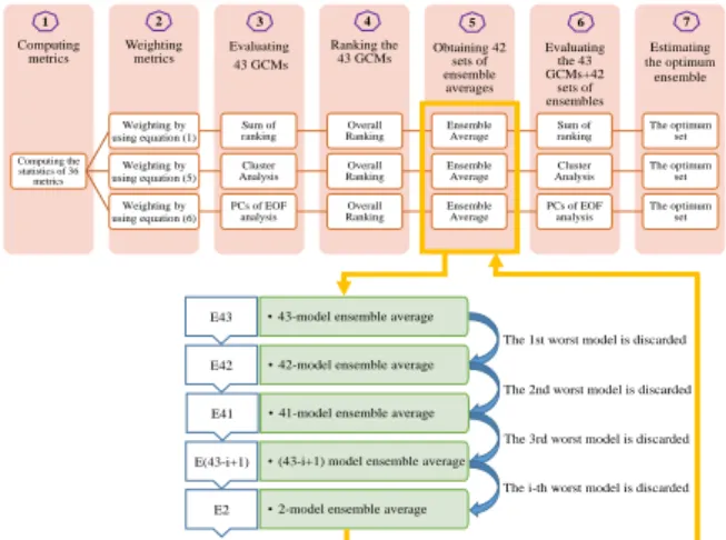
The evaluation framework and ensemble method in this study is illustrated as a flowchart in Figure 1. Firstly, the statistical values of all performance metrics are computed. After weighting metrics based
on different criteria and different way of each evaluation purpose, the combined set of diagnosis performance index is evaluated by using three different criteria, namely summation of rank (SR), Euclidean distance of cluster analysis (CA), and Principal Components of EOF analysis (PC). From the combined set of diagnosis performance index, the overall ranks of the 43 GCMs are obtained based on the three criteria. Then, these ranks are used to make the ensemble averages by dropping the worst model from the averaging one by one (a culling method), and 42 ensemble subsets of each criteria are obtained. After that, the evaluation is performed again for 85 simulation datasets (43 single models plus 42 ensemble subsets) by applying each corresponding criterion used to obtain the overall rankings of the 43 GCMs.
3. Results
The model evaluation and multimodel ensemble estimation were performed for two cases: non-weighted case applying equal weights for all 36 performance metrics and weighted case focusing on the evaluation for agricultural drought monitoring as
• 43-model ensemble average
• 42-model ensemble average
• 41-model ensemble average
• (43-i+1) model ensemble average
• 2-model ensemble average
The 1st worst model is discarded
The 2nd worst model is discarded
The 3rd worst model is discarded
The i-th worst model is discarded E43 E42 E41 E(43-i+1) E2 Estimating the optimum ensemble Evaluating the 43 GCMs+42 sets of ensembles Obtaining 42 sets of ensemble averages Ranking the 43 GCMs Evaluating 43 GCMs Weighting metrics Computing metrics Computing the statistics of 36 metrics Weighting by using equation (1) Sum of ranking Overall Ranking Ensemble Average Sum of ranking The optimum set Weighting by using equation (5) Cluster Analysis Overall Ranking Ensemble Average Cluster Analysis The optimum set Weighting by using equation (6) PCs of EOF analysis Overall Ranking Ensemble Average PCs of EOF analysis The optimum set 1 2 3 4 5 6 7
Figure 1 Diagram of process flow for model
evaluation and ensemble estimation method proposed in this study.
an example, and applied the three criteria to combine a set of diagnostics to create a single performance index.
3.1 Comparison of the three criteria
The results of the model evaluation by the three criteria show very high correlation. The summation of the ranking numbers of the three criteria is computed to select the best single model. The smaller summation value a model has, the better the model performs. Based on this summation of ranking number among the three criteria, the model HadGEM2-CC (#28) is the best single model from the evaluation among the 43 models for the non-weighted case, while the model MPI-ESM-LR (#38) is selected as the best single model for the weighted case.
3.2 The optimum ensemble estimation
The evaluation is performed for 43 GCMs plus 42 subsets of ensembles based on the corresponding criterion from which the ensemble subsets are determined. For these evaluations, we develop a simple graphical illustration of the results which is convenient to visually recognize the optimum ensemble subset or the single GCM; hereafter, it is called decisive graph (not shown). Based on those decisive graphs, we obtain three optimum ensemble subsets from the three criteria for the non-weighted case, namely SR-E9 which coming from nine-model ensemble averaging for SR criterion, CA-E3, and PC-E5. For the weighted case, other three optimum ensemble subsets are also obtained, namely SR-E11, CA-E9, and PC-E8. We notice that there appear three core members of GCMs which always take part in these optimum ensemble subsets, no matter which criterion is used for either the non-weighted or the weighted cases. Moreover, we notice that the members of these optimum ensemble subsets are not sensitive to the choice to criteria used. This result is helpful for practical use because we do not need to be careful to choose the criterion.
3.3 Demonstration of improvement of the optimum ensemble subsets
We demonstrated the improvement of the obtained optimum ensemble subsets for both the non-weighted and the weighted cases in term of the mean state and distribution of the monthly precipitation data over ICR comparing to the best single model or all model ensemble (E43). For the mean state, the optimum ensemble subsets show better spatial structure of the
annual precipitation and average seasonal precipitation than the best single model or all model ensemble (not shown). For the precipitation data distribution, all the optimum ensemble subsets improve on reproducing the basic distribution (mean, range, and quartile) and the Probability Density Function (PDF) of the area-averaged monthly precipitation over ICR than the best single model or the total model ensemble for both the non-weighted and the weighted cases (Figure 2).
4. Concluding Remarks
The model evaluation and ensemble estimation by applying weights on performance metrics introduced in this study provide a reasonable result for an impact assessment purpose. Our method of ensemble estimation is useful to objectively address the question of how many models ensemble is enough for climate change projection studies (Knutti, 2010). In this study, a simple and user-friendly decisive graph for evaluating single model and model ensemble estimation was developed. The climate model evaluation introduced in this study can become a framework for the evaluation of GCMs for multiple perspective of impact assessment over a regional scale.
References
Knutti R., (2010): The end of model democracy? Climate Change, 120, 395-404.
Rupp, D. E., Abatzoglou, T., Hegewisch, K. C., and Monte, P. W., (2013): Evaluation of CMIP5 20th
century climate simulations for the Pacific Northwest USA. Journal of Geophysical Research: Atmospheres, 118, 10884-10906.
Figure 2 Violin plot of area-averaged monthly
precipitation of the APHRODITE (AP), the best single model, total model ensemble (E43), and the optimum ensemble subsets from the three criteria.