CHAPTER ONE
INTRODUCTION AND OVERVIEW OF THE COUNTRIES 1. Introduction
The saving rate of any country is an important indicator of economic development
since the domestic saving rate is directly related with the investment rate and the lending
capacity of the banking system. According to economic theory, in a closed economy,
saving constitutes the only source of investment and the two must be equal by definition.
Conventional wisdom says that in any economy, banking sector accumulates its funds
mainly through the domestic saving. According to Wirvick (1986), domestic saving
originates from three main sectors of the economy, namely government sector, corporate
sector, and the household sector. He points out that the government sector, which consists
of the central and local governments, accumulates funds for saving from its budget surplus.
The corporate sector gets its saving from its own profit. The household sector’s saving
equals its income minus expenditure. He argues that the level of mobilization and
utilization of domestic saving affects economic development for a country.
The rest of the chapter is organized as follows. In the next section, we present the
significance of the study. The third section shows how our study is different from the
previous studies. The fourth section presents an overview of the four countries that are
Chapter organization is given in the final section.
2. Significance and objectives of the study
There are numerous studies on saving behavior for developed countries. But the same is
not true for developing countries. Policy makers have suffered from a dearth of knowledge
regarding the nature of saving behavior in developing countries due to lack of research.
Therefore, the research findings will increase the present knowledge about saving behavior
of the south Asian countries.
The determinants of saving have been receiving attention of economists because
of their significant impact on policymaking. The relationships between economic growth
and saving, income inequality and saving, demographic factors and saving, and
macroeconomic stability and saving have not been studied carefully for South Asia.
Saving is income that part of which is not spent, but put aside for future
consumption. Investment is one of the vital factors for any country for economic
development. The close relationship between saving rate and economic growth is
explained by many economic growth models. The relationships between saving and
investment, and saving and economic growth are highly debatable issues among
economists. These issues have been subject of great interest and debate among economists
for many years.
South Asian countries are economically more integrated with the rest of the world now
than two decades ago. However, South Asia’s export as a percentage of gross domestic
products (GDP) is still low compared to East Asian countries. Also, South Asian countries
have low saving rates compared to many East Asian countries.
In this thesis, we do the following:
(1) Identify the determinants of savings for the South Asian countries.
(2) Measure the degree of international capital mobility for the South Asian countries and
for the region.
(3) Examine whether higher saving rate is a primary determinant of economic growth rate
for the South Asian countries.
(4) Examine whether the low share of trade in GDP is one of the reasons for the low saving
rate in this region.
3. How the study differs from the previous studies
Our study differs from the other existing studies on saving in the following ways.
We carry out a comprehensive study of saving behavior in four major South Asian
countries. In this thesis, South Asian countries mean the major South Asian countries
which are Bangladesh, India, Pakistan and Sri Lanka. We study the determinants of saving,
relationships between saving and investment, between saving and economic growth, and
between saving and investment, they study either an individual country or cross-section of
countries. We analyze saving behavior by using individual country data and panel data.
The relationship between saving and export is an important issue for policy making. But
the relationship has not been studied for South Asian countries. Thus, the study fills a gap
in the literature that has not studied for South Asian countries. Previous studies have not
used impulse response functions to examine the short-run dynamic responses between
saving and GDP for South Asian countries. No previous study has used two
error-correction models to study international capital mobility for an individual country for
the South Asian region.
We use both Jansen (1996) and Johansen cointegration tests to study international
capital mobility. For the South Asian countries, Ng-Perron (2001) and Im et al. (2003) unit
root tests have not been used to test for stationarity for individual country and panel data,
respectively. The Breusch-Godfrey test is more powerful than the Durbin-Watson statistics
to test for serial correlation. The Breusch-Godfrey serial correlation test has not been used
for the South Asian countries to test for serial correlation. We use the vector autoregressive
and moving average processes with exogenous regressors (VARMAX procedure in SAS
program) for the panel cointegration and causality for the South Asian countries and these
4. Overview of the four economies
This section gives an overview of the selected South Asian countries namely, Bangladesh,
India, Pakistan and Sri Lanka. This will be useful in the thesis to analyze the behavior of
saving in South Asian countries. Level of social development, economic structure, GDP,
saving, and investment are briefly pointed out.
4.1. Bangladeshi economy
The People's Republic of Bangladesh is in the northeast of the Indian subcontinent. It has
an area 147,570 sq km with a population about 140 million. When India was partitioned
and the independent dominions of India and Pakistan were created in 1947 by the British
government, present day Bangladesh was in the Pakistani territory. Before the
independence, Bangladesh was called East Pakistan. Almost from the advent of
independence of Pakistan in 1947, there were conflicts between East and West Pakistan.
On March 26, 1971, after a war, people of the East Pakistan became an independent
country. Unfortunately, Bangladesh has faced natural and political disasters since
independence and these natural and political disasters have affected the economic progress.
Economic, social and political ideologies have periodically changed based on
policy stances of political parties since the independence of Bangladesh. According to
Khan et al. (2000), the Bangladeshi government initiated a policy of open economy and
acceleration took place, after the implementation of the project which is called “five-year
financial sector reform project (FSRP)”. Bangladesh Bank (2005) points out that the
present government is committed to promote the market economy and to pursue policies
for supporting and encouraging private investment and eliminating unproductive
expenditures in the public sector.
4.1.1. Degree of social development
Despite its steady GDP growth rate from 1990 to 2004, Bangladesh has not achieved
sufficient progress in the fields of health, education, and social welfare. According to the
Bangladesh Bank (2004), poverty is one of the main problems in the country. Urban and
rural poverty is increasing while income inequality is alarmingly increasing throughout the
country. World Bank (2005) points out that nearly half of the population in Bangladesh are
living in deprivation and with inadequate health facilities. Table 1.1 shows some key
indicators of development of Bangladesh and some selected industrial countries.
According to the indicators such as malnutrition and maternal mortality rates,
Bangladesh remains among the least developing countries in the world. Higher
unemployment rate also makes it harder for the Bangladeshi government to achieve its
goal such as reduction of poverty and income disparity. Though social development
indicators paint gloomy picture, there has been a sharp fall in the rate of population growth
Table 1.1: Some key indicators of development for South Asian and other selected developed countries Life Expectancy at Birth Country Gini Index Male Female Adult Literacy Rate Average Annual Population Growth Rate Australia 0.32 77 83 -- 1.2 Japan 0.25 78 85 -- 0.2 Singapore 0.43 76 80 93 1.9 Bangladesh 0.31 62 63 41 1.7 India 0.33 63 64 61 1.5 Pakistan 0.27 63 65 49 2.4 Sri Lanka 0.38 72 76 90 1.3 UK 0.34 75 80 -- 1.2 USA 0.38 75 80 -- 1.0
Source: World Bank (2005)
4.1.2. Economic structure
Bangladesh is an agricultural country. Major agricultural products are rice, jute, wheat,
population is engaged in farming. Garment & apparel, jute, leather, and tea are the
principal sources of foreign exchange. As most of the developing countries did after
independence, Bangladesh had socialism as the economic ideology with a dominant role of
the public sector. But, since the mid-eighties, Bangladesh has pursued economic reforms
towards establishing a market economy with an emphasis on private sector oriented
economic growth.
Economists often use a change in sectoral composition of GDP away from
agricultural sector toward manufacturing and services sector as a measure of economic
development. Figures 1.1 and 1.2 show that in Bangladesh, the sectoral composition of
GDP has moved away from agricultural sector to manufacturing and service sectors. The
agricultural sector’s contribution to GDP has fallen from 32 percent in 1980 to 22 percent
in 2004.
Figure 1.1: Sectoral composition of GDP at factor cost in 1980 for Bangladesh A g ric u lt u re , va lu e a d d e d (% o f G D P ) 3 2 % In d u s t ry , va lu e a d d e d (% o f G D P ) 2 1 % S e rvic e s , va lu e a d d e d (% o f G D P ) 4 7 % A g ric u lt u re , va lu e a d d e d (% o f G D P ) In d u s t ry , va lu e a d d e d (% o f G D P ) S e rvic e s , va lu e a d d e d (% o f G D P )
Figure 1.2: Sectoral composition of GDP at factor cost in 2004 for Bangladesh Agriculture, value added (% of GDP) 21% Industry, value added (% of GDP) 27% Services, value added (% of GDP) 52%
Agriculture, value added (% of GDP)
Industry, value added (% of GDP)
Services, value added (% of GDP)
Source: International Monetary Fund (2005)
According to Bank of Bangladesh (2003), the current account deficit was 2.5 percent of
GDP in 2002. Figure 1.3 shows that the trade balance has become more negative since
independence.
Figure 1.3: Balance of trade for Bangladesh, 1975-2005
-3000 -2500 -2000 -1500 -1000 -500 0 197 7 198 0 1983 198 6 1989 1992 199 5 1998 200 1 200 4 Trade Balance
Recently, the government has taken various steps to increase foreign exchange reserves.
Some of the measures are punitive measures against illegal foreign exchange transactions,
introduction of incentives to encourage overseas workers to send their remittances through
official channels, closer monitoring of imports to discourage the practice of over invoicing,
and encouragement of repatriation of export earnings.
4.1.3. Gross domestic product
Unfortunately, in Bangladesh one of the major barriers to growth is frequent cyclones and
floods. Also, inefficient state-owned enterprises, inadequate port facilities, a rapidly
growing labor force that cannot be absorbed by the agricultural sector are impediments to
economic development. It is a common knowledge that many development efforts in the
developing countries have turned into exercises in futility because of the inefficiency and
corruption among both politicians and bureaucrats. Bank of Bangladesh (2003) points out
that though a number of measures have been taken to increase economic growth, the
corruption of the public sector has set back the progress.
Figure 1.4 shows that except for 1971, 1972, and 1975 Bangladesh had a positive
GDP growth rate since independence. GDP growth rate of Bangladesh was negative in
1975 because of the civil unrest and bad weather. The GDP growth rate increased after
1975. The average GDP growth rate was 3.7 percent until the late 1990s. According to the
2001, terrorist attack, slowed down the GDP growth in 2002. It was 3 percent in 2002.
However, the GDP growth rate increased in 2003, due to a rise in both domestic and
external demand.
Figure 1.4: GDP growth rate for Bangladesh, 1971-2005
-20 -15 -10 -5 0 5 10 15 1971 1974 1977 1980 1983 1986 1989 1992 1995 1998 2001 2004 GDPG
Source: Source: International Monetary Fund (2005)
Because of progress of the agricultural and the industrial sectors, the economy has
maintained an upward trend of GDP growth rate, despite external economic and internal
political pressures since 1990. Since 1990, Bangladesh has been having an average 5
percent GDP growth rate. The country has achieved considerable economic progress over
the past few years. If Bangladesh is able to eliminate corruption and inefficiencies in the
government sector, and improve economic governance, it could achieve a higher rate of
4.1.4. Saving and investment
Bangladesh has had a low saving rate compared to other countries in the South Asian
region since its independence. Figure 1.5 shows that there has not been a consistent
increase in saving and investment rates for Bangladesh. However, in recent years, these
rates have increased. The saving rate increased from 2.97% in 1976 to 18.38% in 2003.
The figure shows that there was a steep decline of the saving rate during the period from
1970 to 1976. Bangladesh had an upward trend in the saving rate since 1979 although there
have been considerable fluctuations around the trend. According to the Bank of
Bangladesh (2001), remittances from expatriates and workers who are temporarily abroad
have contributed to the growth in the saving rate in recent years. This is also the case for
other countries in South Asia. According to the Bank of Bangladesh (2002), in recent years,
the national saving rate has been much higher than the domestic saving rate because the
balance in the current account has been positive.
Figure 1.5: Saving-investment gap for Bangladesh, 1960-2004
-5 0 5 10 15 20 25 30 19 60 19 63 19 66 19 69 19 72 19 75 19 78 19 81 19 84 19 87 19 90 19 93 19 96 19 99 20 02 Year %
Gross capital formation (% of GDP)
Gross domestic savings (% of GDP)
Investment-saving gap (% of GDP)
Since independence, public investment rate has been much less than private
investment rate for Bangladesh. According to the Bank of Bangladesh (1990), investment
was about 17 percent of GDP in which shares of public and private sectors were about 7
percent and 10.27 percent, respectively in the late 1980s. The investment rate has been
increasing since the early 1990s and it rose to 23.4 percent of GDP in the early 2000. Out
of the total investment, shares of public and private sector contributions were about 6 %
and 17% respectively in 2003. Bank of Bangladesh (2001 and 2002) points out that
because of the private sector-oriented reforms in Bangladesh, domestic investment and
foreign direct investment have been increasing in the past decade.
The investment-saving gap was widening during the period from the early 1960s
to the late 1980s. Since the early 1990s saving rate has been increasing and thus, the gap
between saving and investment rates has reduced. Table 1.3 shows that Bangladesh’s
saving rate is low compared to that of East Asian and Latin American countries during the
period from 1975 to 1985.
4.2. Indian economy
India’s history begins not with its independence which was achieved in 1947, but more
than 4500 years ago. When India became independent, present-day Pakistan and
Bangladesh were within its territory. India has an area of 3,165,596 sq km and a population
India gained political freedom, the country was suffering from poverty and low standard of
living. As a common feature for all the countries that gained independence after being
colonized for a long period, agriculture was the principal industry at independence.
According to Sankaran (1984), agriculture, forestry, and fishing accounted for 60 percent
of the GDP and for a much larger proportion of employment. Manufacturing was
dominated by the jute and cotton textile industries. The two industries accounted for about
10 percent of GDP. The great challenge that India faced after the independence was to
eradicate poverty and to restructure the stagnant economy.
As many other developing countries in the South Asian region, India emphasized
centrally planned economic policies for many years after independence. Soon after the
independence, the government emphasized self-sufficiency rather than international trade
and imposed strict controls on foreign exchange as well as on import and export. As
Delong (2001) emphasizes, in 1991, India launched a series of economic reforms because
of a foreign exchange crisis and the slowdown of economic growth. The economic reforms
and restructuring programs consisted of liberalization of the exchange rate, foreign direct
investment, and financial market. Also, the policy reforms included significant reductions
in tariffs and other trade barriers, and significant adjustments in government monetary and
fiscal policies. As a result of the policy reforms, the Indian economy is progressing well.
foreign direct investment and a growing middle class of 150-200 million which has
disposable income for a comfortable life.
4.2.1. Degree of social development
Economic development is a multi-dimensional phenomenon. GDP growth, income
inequality, level of education, level of nutrition, literacy rate, access to the health facility,
and availability of housing are some of its important dimensions. According to Sankaran
(1984), though India has increased its GDP growth rate, there is a wide socio-economic
disparity.
There is a widespread disparity in terms of economic development among the
states in India. Though the economy is progressing well, the benefit of the rapid economic
growth has not reached all parts of the country. Table 1.1 compares some key social
development indicators of India with some developed countries.
Reserve Bank of India (2002 and 2003) opines that income distribution has not
changed much even after the economic reforms in the early 1990s. Even now, the majority
of the Indian people have low standard of living and many families live just above the
subsistence level. According to the Reserve Bank of India (2005), a majority of the people
who are above the poverty line, is still poor enough to qualify for poverty elimination
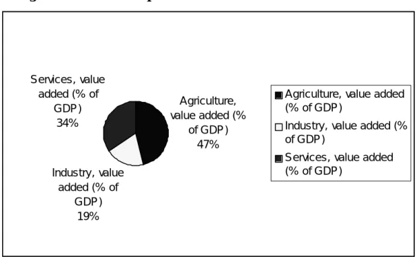
4.2.2. Economic structure
At independence, the economy was dominated by agricultural activities. Agricultural value
added as a percentage of GDP was more than 50. Figure 1.6 shows the sectoral
composition of GDP in 1960. The figure shows that even after the fist decade of
independence, the economy was heavily dependent on agricultural activities.
Figure 1.6: Sectoral composition of GDP at factor cost in 1960 for India
Agriculture, value added (% of GDP) 47% Industry, value added (% of GDP) 19% Services, value added (% of GDP) 34%
Agriculture, value added (% of GDP)
Industry, value added (% of GDP)
Services, value added (% of GDP)
Source: International Monetary Fund (2005)
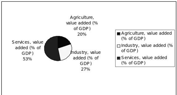
Until the late 1970s the economy was controlled heavily by the government.
Beginning in the late 1980s, India has started to liberalize its economy. As a result of the
economic reforms, agricultural sector’s contribution to GDP has fallen and industry and
service sectors’ contribution to GDP has increased. Figure 1.7 shows the sectoral
Figure 1.7: Sectoral composition of GDP at factor cost in 2004 for India
A gric ulture, value added (%
of GDP ) 20%
Indus try , value added (% of GDP ) 27% S ervic es , value added (% of GDP ) 53%
A gric ulture, value added (% of GDP )
Indus try , value added (% of GDP )
S ervic es , value added (% of GDP )
Source: International Monetary Fund (2005)
Compared to many other developing countries, India has not faced a persistent
balance of trade problem. However, in the late 1980s, India was relying heavily on foreign
borrowing to finance its development plans. Moreover, in the early 1990s, the world oil
prices increased very sharply. As a result of the heavy foreign borrowing and high oil price,
Indian government faced a severe balance of trade crisis.
The government embarked on a series of economic reforms to overcome the
situation. Since then, foreign portfolio and direct investment flows have risen significantly
and have contributed to healthy foreign currency reserves. Figure 1.8 shows the
Figure 1.8: Government debt as a percentage of GDP, 1955-2004 0 1 0 2 0 3 0 4 0 5 0 6 0 19 55 19 59 19 63 19 67 19 71 19 75 19 79 19 83 19 87 19 91 19 95 19 99 D e bt: D o m e stic as a G D P% D e bt:Fo re ign as a G D P%
Source: International Monetary Fund (2005)
Most of the developing countries have the problem of existence of two separate
economic systems within one country. This is called the dual economy problem. According
to the Reserve Bank of India (2004), the Indian economy also has the so-called dual
economy problem. In India, there is an informal or an unorganized, sector that is largely
rural and it consists of farming, fishing, forestry, and cottage industries. The formal modern
sector includes large-scale manufacturing and mining, major financial and commercial
businesses, and telecommunications.
Although it has the dual economy problem, one should not overlook the progress
India has achieved in the service sector especially in the field of information technology.
India is one of the fine examples of how information technology (IT) would bring
role as the enabler and accelerator of economic development. Reserve Bank of India (2003
and 2004) points that the economy is positively influenced by IT and software
development sectors that has recently ridden the outsourcing boom. India has achieved a
big niche in the international marketplace for IT products by using the low wages of its IT
workers.
Reserve Bank of India (2005) points out that the U.S. has been the largest trading
partner of India in the recent past. At present, textiles and ready-made garments,
agricultural and related products, gems and jewelry, leather products, and chemicals are the
main exports of India while aircraft and parts, advanced machinery, fertilizers, ferrous
waste and scrap metal, and computer hardware are the main imports.
4.2.3. Gross domestic product
At independence, India had a lot of problems such as the war with Pakistan, lack of human
resources, and poverty. However, now, India has a higher GDP growth rate than other
countries in South Asia. Figure 1.9 indicates that during the 1950s, the average GDP
growth rate was 4.5 percent. But after 1960, India’s GDP growth rate fell dramatically.
DeLong (2001) points out that many factors had contributed to the slowdown of the
economy after the mid-1960s. DeLong argues that in India, structural deficiencies, such as
the lack of institutional changes in agriculture and the inefficiency of the industrial sector,
1962 and with Pakistan in 1965 and 1971, respectively, currency devaluation in 1966, the
first world oil crisis in 1973-74, and adverse weather conditions were also responsible for
the low GDP growth rate. Figure 1.9 shows that the GDP growth rate was negative in
1979.
Figure 1.9: GDP growth rate for India, 1960-2005
GDPG -8 -6 -4 -2 0 2 4 6 8 10 12 1961 1965 1969 1973 1977 1981 1985 1989 1993 1997 2001 Year % GDPG
Source: International Monetary Fund (2005)
The GDP growth rate increased in the 1980s. During 1980-1989, the economy
performed better and GDP grew at an annual rate of 5.5 percent. During the period, Indian
industry grew at an annual rate of 6.6 percent and agriculture at a rate of 3.6 percent. As
DeLong (2001) explains, high rate of investment was a major factor for the GDP growth in
the late 1980s. The balance of trade crisis of 1990 and the subsequent radical policy
changes led to a temporary decline in the GDP growth rate, which fell from 6.9 percent in
has been one of the fastest growing economies in the South Asian region and the world.
This acceleration in the economic growth is mainly because of the policy changes that have
been initiated since 1991.
4.2.4. Saving and investment
Over the past four decades, Indian saving rate has been consistently increasing though
there are some fluctuations from year to year. The saving rate shows an upward trend from
1960 to 2004 although there are considerable fluctuations around the trend. The saving rate
was about 10% of GDP in the early 1950s. It was about 17% in the early 1970s and it was
about 25% in the late 1980s. According to the Reserve Bank of India (2005 and 2006),
foreign remittances from Indian emigrants have increased since the late 1990s.
Remittances from expatriates and others working abroad temporarily have contributed to
the higher saving rate in the recent years. Wolf (2005) point outs the economic reforms
which were initiated in the early 1990s have affected the saving rate in India. At present,
the saving rate is about 30%.
The main feature of Indian saving has been the dominant role of private saving
during the period from 1960 to 2004. While the private saving rate has shown an
increasing trend since 1960, public saving rate, which consists of saving by government
administration, government departments and public enterprises, has shown a declining
from about 8% in the early 1950s to 15% in the 1970s and to 25% in the late 1990s. The
private saving rate has shown a much faster growth since the 1970s.
Table 1.2 shows that India’s saving rate is the highest among the South Asian
countries and it was much higher than many of the East Asian countries during the 1960s.
By the mid 1990s, when most of the East Asian countries achieved high economic growth
rates, Indian saving rate was lower than that of many East Asian countries. In Latin
America, countries such as Venezuela and Peru had a high saving rate than that of India.
Since independence, the investment rate has shown an upward trend for India.
However, Figure 1.10 shows that there are some fluctuations around the trend. The
investment rate increased from 12% in the early 1960s to around 15% in the late 1970s and
to 25% by mid-1990. It was around 23% in the early 2000. A narrow saving-investment
gap has been one of the main features of the Indian economy.
Figure 1.10: Saving-investment gap for India, 1960-2004
-5 0 5 10 15 20 25 30 196 0 196 3 196 6 196 9 197 2 197 5 197 8 198 1 198 4 198 7 199 0 199 3 199 6 199 9 200 2 Year %
Gross capital formation (% of GDP)
Gross domestic savings (% of GDP)
Investment-saving gap (% of GDP)
Table 1.2: Average saving rate as a percentage of GDP for selected countries South Asia 1960-64 1965-69 1970-74 1975-79 1980-84 1985-89 1990-94 1995-99 2000-04 Bangladesh NA NA NA 1.5 1.9 2.9 12.0 14.6 17.5 India 14.3 15.0 17.4 20.8 19.3 20.8 22.4 21.7 22.1 Pakistan 10.5 11.8 8.7 7.3 7.9 9.6 15.4 14.8 14.2 Sri Lanka 11.9 10.4 13.5 13.8 13.7 11.6 14.8 17.3 15.8 East Asia China 33.2 33.0 33.5 32.6 34.3 35.2 39.7 42.1 43.6 Hong Kong 20.9 25.8 29.3 32.3 31.7 35.0 33.4 29.7 31.5 Indonesia 10.0 5.6 20.7 28.1 31.6 29.3 32.7 27.6 22.8 Korea 4.4 13.0 17.5 25.3 26.9 35.6 34.9 36.2 31.9 Malaysia 23.8 24.4 26.9 32.5 31.6 34.6 36.8 44.5 43.3 Singapore 4.3 14.9 24.0 33.2 42.7 41.0 45.4 51.1 45.8 Thailand 16.4 21.3 22.6 21.9 23.8 29.1 35.5 35.1 31.3 Latin America Argentina 22.1 23.7 23.7 30.6 23.5 21.2 16.9 17.1 22.0 Brazil 19.8 20.3 20.1 21.5 20.9 25.5 21.6 19.1 21.8 Chile 15.2 20.0 16.3 17.3 14.3 25.3 26.0 24.5 25.6 Costa Rica 14.4 13.0 14.6 16.1 22.9 23.7 15.9 16.6 18.3 El Salvador 12.4 11.0 14.3 18.8 8.2 5.7 2.8 4.5 1.3 Haiti 5.2 3.1 9.0 7.3 6.2 4.9 1.0 6.2 4.1 Jamaica 26.0 28.1 21.5 15.0 14.0 19.7 22.8 16.9 13.0 Mexico 16.1 18.2 18.1 20.3 27.1 23.6 18.9 23.5 19.2 Nicaragua 15.1 15.8 16.5 15.5 6.3 4.6 6.3 6.7 10.0 Paraguay 12.6 12.8 15.8 21.6 18.8 20.6 12.5 7.5 9.7 Peru 38.0 29.2 17.1 18.0 28.5 21.5 16.4 18.8 18.6 Uruguay 18.2 19.4 18.0 18.9 16.0 17.3 16.5 14.9 14.2 OECD Countries Canada 21.7 25.2 24.9 24.1 24.3 23.3 19.1 22.9 25.2 France 28.0 28.9 27.3 24.2 20.4 20.8 21.2 21.0 21.7 Italy 36.4 25.3 25.5 26.1 23.6 22.8 21.6 22.9 20.8 Japan 34.4 36.3 38.6 32.7 31.1 32.5 32.5 29.1 26.0 UK 18.1 20.0 19.9 20.3 18.7 18.1 15.8 16.6 14.0 United States 19.6 20.2 19.6 19.8 18.9 16.8 16.2 17.6 14.9 Source: World Bank (2006)
Figure 1.10 shows that except for 1991 and 1993, the investment rate has been higher than
the domestic saving rate in India. The saving-investment gap has been consistently less
than 3.5 as a percentage of GDP in India from 1960 to 2003.
4.3. Pakistani economy
Pakistan became an independent country in 1947. It has an area of about 796,000 sq. km
with an estimated population of 152.1 million. Its population density is 197 persons per sq.
km. Pakistan is the sixth most populous country in the world. Since its independence,
Pakistan faced a number of challenges on the political and economic fronts. Pakistan is a
politically unstable country. It has suffered from decades of internal political disputes and
confrontations with the neighboring India. Monshipouri and Samuel (1995) point out that
the three military leaders who governed Pakistan, implemented martial law to govern the
country. Under these military regimes, the socio-economic development was low and
problems such as poverty, income inequality, unemployment, and inflation were not
attended to.
Pakistan followed import substitution policies until the late 1980s. Monshipouri
and Samuel (1995) point out that import substitution policies that were pursued by the
governments since independence were imprudent and led to a slowdown of economic
growth in Pakistan in the 1990s. From 1990, the government has started to follow an open
implementing substantial macroeconomic reforms since 2000, after being advised by the
International Monetary Fund (IMF). Since 2000, the government has begun to remove
barriers to foreign trade and investment, reform the financial system, ease foreign
exchange controls, and privatize state-owned enterprises.
4.3.1. Degree of social development
Partially due to the low growth rate, Pakistan has achieved very low progress in social and
human development.
No more than 45.7 percent of adults are literate, and life expectancy is about 63
years. The population is growing at over 2.4 percent annually which is very close to
average real GDP growth rate since independence. According to State Bank of Pakistan
(2004), poverty and income inequality are the major problems.
Table 1.1 compares some key social development indicators of Pakistan with that
of some developed countries. In Pakistan, inadequate provision of social services such as
health, education and high annual population growth rate have contributed to a persistence
of poverty and income disparity.
4.3.2. Economic structure
At independence, agricultural activities accounted for 46 percent of GDP in Pakistan. Its
principal natural resources are arable land, water, and extensive natural gas reserves. The
After the introduction of the open economy policy, the GDP growth rate has accelerated in
the recent past. Also, Pakistan's industrial and service sectors are experiencing a rapid
growth. At present, Pakistan receives its foreign exchange mainly from the textile industry. Figure 1.11: Sectoral composition of GDP at factor cost in 1960 for
Pakistan Agriculture, value added (% of GDP) 46% Industry, value added (% of GDP) 16% Services, value added (% of GDP) 38%
Agriculture, value added (% of GDP)
Industry, value added (% of GDP)
Services, value added (% of GDP)
Source: International Monetary Fund (2005)
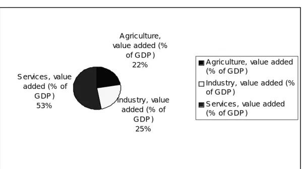
Figure 1.12: Sectoral composition of GDP at factor cost in 2004 for Pakistan
A gric ulture, value added (%
of GDP ) 22%
Indus try , value added (% of GDP ) 25% S ervic es , value added (% of GDP ) 53%
A gric ulture, value added (% of GDP )
Indus try , value added (% of GDP )
S ervic es , value added (% of GDP )
The textile industry is responsible for over 64 percent of the country's exports. Growth of
non-agricultural sectors such as industry and service sectors has changed the structure of
the economy, and at present, agricultural value added to GDP is one-fifth of GDP. Figures
1 and 2 show sectoral composition of GDP for Pakistan in 1960 and 2004, respectively.
The current account deficit is an important indicator for any country to gauge the
pressure on a country’s external sector. According to State Bank of Pakistan (2003 and
2004), a persistent current account deficit has led to a depreciation of the Pakistani rupee.
Economic mismanagement and fiscally imprudent economic policies caused a large
increase in the public debt and led to fall in the foreign currency reserves in the 1990s.
Figure 1.13 shows the balance of trade in Pakistan.
Figure 1.13: Balance of trade for Pakistan, 1976-2004
- 4 0 0 0 - 3 5 0 0 - 3 0 0 0 - 2 5 0 0 - 2 0 0 0 - 1 5 0 0 - 1 0 0 0 - 5 0 0 0 1 976 1979 1982 1985 1988 1991 1994 1997 2000 2003 Y e ar A s a G D P % Trade B alan c e
Source: International Monetary Fund (2005)
was estimated to be about 260% of the value of exports of goods and services (State Bank
of Pakistan, 2003). This is far in excess of the commonly accepted benchmarks for
sustainability, which fall in the range of 150–200%. State Bank of Pakistan (2003) shows
that in the recent years, FDI inflows have fallen, because of Pakistan's tense relationship
with India. Fallen in FDI would put more pressure on the economy and would further
deteriorate the balance of trade.
4.3.3. Gross domestic product
During first decade after independence, Pakistan made good economic progress because it
had relatively peaceful social and political situations. The average annual GDP growth rate
was about 3.5 percent until mid 1960s. Figure 1.14 shows that GDP growth rate was 6
percent per year during 1980-1990, but it decreased after 1997. State Bank of Pakistan
(2000) argues that GDP growth rate fell after 1997 due to the financial crisis in Asia.
Figure 1.14: GDP growth rate for Pakistan, 1954-2004
-6 -4 -2 0 2 4 6 8 10 195 4 195 8 196 2 196 6 197 0 197 4 197 8 198 2 198 6 199 0 199 4 199 8 200 2 Year % GDPG
According to the State Bank of Pakistan (2004), the government hopes to achieve a 8
percent GDP growth rate by the end of 2010.
4.3.4. Saving and investment
Pakistan’s saving rate is about 12 %. This is one of the lowest in Asia for the period for
2000-2004. The saving rate showed a downward trend from 1967 to 1986. However, from
1987 to early 1990s, there was an upward trend in the saving rate. Once again, Pakistan’s
saving rate shows a downward trend from the mid-1990s. According to the State Bank of
Pakistan (2004), the national saving rate in Pakistan has been lower than the domestic
saving rate for most years because of the negative balance in the current account. The State
Bank of Pakistan (2004) points out that private saving rate has been increasing while
public saving rate had been declining during the period from 1960 to 2003.
Figure 1.15: Saving-investment gap for Pakistan, 1967-2004
0 5 10 15 20 25 1 967 1970 1973 1976 1979 1982 9851 1988 1991 1994 1997 2000 2003 Year %
Gross capital formation (% of GDP)
Gross domestic savings (% of GDP)
Investment-saving gap (% of GDP)
Source: World Bank (2006)
countries over the period from 1965 to 2004. For 1960-1964, Pakistan’s saving rate was
much higher than that of Singapore, Korea and Indonesia. From the late 1960s, Pakistan’s
saving rate has been lower than that of all East Asian countries. Among the four South
Asian countries, Pakistan’s saving rate is now only higher than that of Bangladesh. In Latin
America, saving rates of all most all the countries have been consistently higher than that
of Pakistan from 1960 to 2004, except for Haiti.
Pakistan has a relatively modest investment rate. There has not been a consistence
increase in the investment rate for Pakistan. Investment rate in Pakistan decreased from the
late 1960s to the early 1990s and then increased from the late 1990s. Figure 1.15 shows
that the investment-saving gap has reduced during the period from 1967 to 2004.
According to the State Bank of Pakistan (2004), the current investment rate is inadequate
for both current and future needs of economic growth for Pakistan.
4.4. Sri Lankan economy
Sri Lanka is a small island with a population about 19.1 million and a landmass of 65,525
km2. It is located below India in the South Asian region. Sri Lanka is a democratic country.
The island was known as Ceylon until 1972. It had been colonized by various Western
nations for more than 500 years. Sri Lanka regained its independence in 1948. Until the
late 1970s, Sri Lanka had a planned economic. Sri Lanka started its program of
and introduced export-oriented policy in 1978.
Unfortunately, since the early 1980s, Sri Lanka has experienced an ethnic conflict.
This has led to a huge government budget deficit. Economic progress of the country has
been badly affected by the war. As Lakshman (1997) indicates, if there were no civil war,
Sri Lanka would likely be one of Asia’s top economic performers.
4.4.1. Degree of social development
Although Sri Lanka has low economic growth, it has performed well in terms of social
indicators. The government has been emphasizing social welfare in its economic
development strategies since independence. As a result, it has achieved higher social
development level compared to other developing countries.
According to the Central Bank of Sri Lanka (2004), Sri Lanka had a literacy rate
of 90%, a school enrolment ratio of 97%, and a life expectancy of 73.1 years in 2004. Most
of these social indicators of development are much higher than those in other countries
with similar per capita income levels as Sri Lanka. Table 1.1 shows some key indicators of
social development of Sri Lanka and some selected industrial countries.
4.4.2. Economic structure
The economy was heavily dependent upon agricultural export during independence.
According to Lakshman (1997), until the early 1980s agricultural sector accounted for
Tea, which is famous all over the world, is the main export crop and principal foreign
exchange earner even today. Figure 1.16 shows the sectoral composition of GDP in 1960.
Figure 1.16: Sectoral composition of GDP at factor cost in 1960 for Sri Lanka
A gric ulture, value added (%
of GDP ) 32%
Indus try , value added (% of GDP ) 20% S ervices, value added (% of GDP ) 48%
A gric ulture, value added (% of GDP )
Industry, value added (% of GDP )
S ervic es , value added (% of GDP )
Source: International Monetary Fund (2005)
Figure 1.17: Sectoral composition of GDP at factor cost in 2004 for Sri Lanka
A gric ulture, value added (%
of G DP ) 18%
Indus try , value added (% of G DP ) 27% S ervic es , value added (% of G DP ) 55%
A gric ulture, value added (% of G DP )
Indus try , value added (% of G DP )
S ervic es , value added (% of G DP )
The government has undertaken measures to diversify the economic structure since the
early 1980s. As a result, contribution of the agricultural sector to GDP has fallen during the
past few years. Figure 1.17 shows the sectoral composition of GDP in 2004.
The existence of the dual economy has been one of the main problems since
independence. The dual economy consists of a modern export oriented sector and a
traditional subsistence sector. These two sectors have minimal interrelationships. The
export oriented sector deals with plantations, transport, communication, banking, and
garment and apparel. The traditional sector consists of peasant agriculture, small scale
fishing, cottage industry, and informal service sector. According to the Central Bank of Sri
Lanka (2004), at present, Sri Lanka’s most dynamic sectors are textile and apparel, food
and beverage, telecommunication, and insurance and banking, and food processing.
Figure 1.18: Government debt as a percentage of GDP for Sri Lanka, 1973-2004
0 20 40 60 80 100 120 1 973 1976 1979 1982 1985 9881 1991 1994 1997 2000 2003 Year % D omestic as GD P% Foreign as GDP%
Sri Lanka has been having a persistent balance of trade problem. The country is
dependent on large amounts of foreign aid and loans. Figure 1.18 shows the government
domestic and foreign debt as a percentage of GDP. However, according to Central Bank of
Sri Lanka (2004), most of the foreign loans are from bilateral agreements and thus, cost of
the foreign loans is low.
4.4.3. Gross domestic product
Until late 1970s, the public sector contributed to GDP more than the private sector. Since
1977, the government has attempted to downsize and to privatize the public enterprises. As
a consequence, the government’s role as a producer has diminished since 1977. Though the
ethnic conflict has affected the economy, Sri Lanka has been having a positive GDP
growth rate since independence except for 1973 and 2001.
Figure 1.19: GDP growth rate for Sri Lanka, 1961-2004
% - 4 - 2 0 2 4 6 8 196 1 196 5 196 9 197 3 197 7 198 1 198 5 198 9 199 3 199 7 200 1 Y e ar GD P Gro w th Rate
Because of the sustained economic growth, coupled with average population
growth of only 1.1%, has pushed Sri Lanka from the ranks of the poorest countries up to
the middle income countries in the recent past. Figure 1.19 shows the GDP growth rate in
Sri Lanka.
From 1950 to 1977, when Sri Lanka heavily relied on agricultural products, it had
an annual GDP growth rate of 4.6 per cent. GDP grew at an average rate of 5.5% in the
early 1990s. But in the late 1990s, due to a drought and ethnic violence GDP growth rate
fell to 3.8%. In 2001, Sri Lanka for the second time in its history experienced a negative
GDP growth rate of -1.4%, because of many reasons such as power shortage, severe
budgetary problem, the global slowdown, and continuing civil conflict. However,
economic growth recovered to 4.0% in 2003 and to 5.2% in 2004.
4.4.4. Saving and investment
Figure 1.20 shows the trends of domestic saving rate, investment rate and gap between
saving and investment rates for Sri Lanka. Though there had been a decline in the size of
the gap between saving and investment rates in the late 1990s, Sri Lanka has a much
higher gap than other South Asian countries. Central Bank of Sri Lanka (2004) points out
that the public sector’s contribution to domestic saving was almost equal to zero or
negative during the period from 1965 to 2003. Except for a few years from 1965 to 2003,
Except for a few years, the national saving rate has been higher than the domestic
saving rate, because of net private transfers from abroad has been positive for most of the
years. Figure 1.20 shows that the investment-saving gap for Sri Lanka has reduced since
the late 1980s. According to the Central Bank of Sri Lanka (2002), a proportion of the
investment-saving gap is financed by private remittances from Sri Lankans who are living
abroad. Private remittances have been increasing continuously since 1996. It increased
from 5.5% of GDP in 1996 to 6.8% of GDP in 2002.
Figure 1.20: Saving-investment gap for Sri Lanka, 1965-2005
-5 0 5 10 15 20 25 30 35 40 19 65 19 68 19 71 19 74 19 77 19 80 19 83 19 86 19 89 19 92 19 95 19 98 20 01 20 04 Year %
Gross capital formation (% of GDP)
Gross domestic savings (% of GDP)
Investment-saving gap (% of GDP)
Source: World Bank (2006)
The average investment rate had been about 14% from 1965 to 1975. There was
an upward trend during the period from 1965 to 1977. According to Lakshman (1997),
from 1965 to 1977, state sponsored activities expanded in many sectors and the share of
public investment averaged more than 40% percent of the total investment. The
the economic reforms, the share of public investment gradually decreased. At present, the
share of public investment is less than 25% of the total investment. Soon after the
economic reforms, investment rate increased to 18%. This sharp increase was mainly
because the private sector increased its contribution to gross capital formation. Because of
the civil conflicts, investment rate has been showing a downward trend in Sri Lanka since
the 1980s.
For the period from 1965 to 2003, the saving rate had been about 14% which was
lower than that of many East Asian or OECD countries. In South Asia, saving rate of Sri
Lanka is slightly higher than that of Pakistan and Bangladesh. Until 1964, the saving rate
was higher than that of Singapore, Korea and Indonesia. Table 1.3 shows that in Latina
America, most of the countries have a higher saving rate than Sri Lanka.
5. Data and methodologies
Data are from two sources for the study. The sources are the World Development Indicators
of the World Bank and the International Financial Statistics of the International Monetary
Fund. Time span is different for the countries because of non-availability of data. We use
different time periods for the four countries based on data availability.
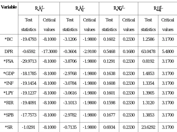
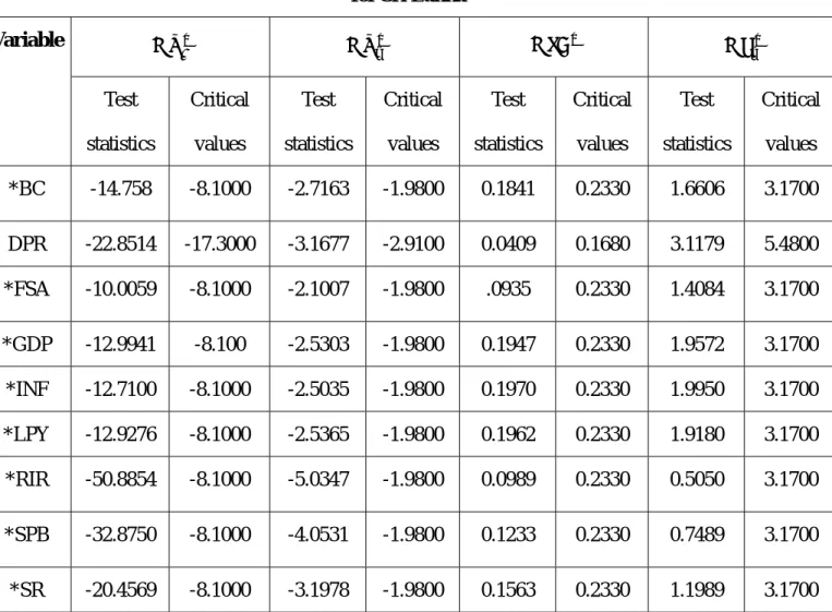
We study the unit root properties of the variables using Ng-Perron unit root tests.
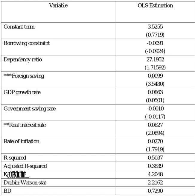
OLS and the fixed effects panel least squares (PLS) are used for regression analysis for
investment, we use both the error correction model that was used by Jansen (1996) and the
Johansen cointegration tests. The Johansen cointegration tests are used to study the
relationships between saving and GDP, and saving and export. For the individual country
studies, if the variables are found to be cointegrated, we use the augmented Granger
causality test. If the variables are not cointegrated, but stationary, the standard Granger
causality tests are performed. We use the VARMAX procedure in the SAS program for the
panel Granger causality tests. The impulse responses are studied by using Cholseky
ordering. For the panel data, we use the panel cointegration test which is presented by
Larsson et al. (2001).
6. Organization of the thesis
The reminder of the thesis is organized as follows. An overview of growth theories and
methodologies for individual country studies are discussed in chapter two. Also, the
chapter deals with methodologies for the panel study, panel regression, and causality and
cointegration tests. In the third chapter, we present a brief literature review, the theoretical
relationship and the empirical results on the determinants of saving. The literature on
saving-investment, the theoretical relationship between saving and investment, and the
empirical results are discussed in chapter four. The fifth chapter has the literature review
and the empirical findings for the relationship between saving and economic growth. The
empirical results of the relationships between saving and investment, and saving and
economic growth. The determinants of saving rate for the panel study are discussed in this
chapter. The seventh chapter presents the results of the relationship between saving and
export for the individual and panel studies. It includes a brief literature review on the
relationships between saving and export. The regression results of the two saving functions
i.e. the Keynesian and the Maizels’ for the four South Asian countries are presented. The
conclusion and summary of the findings are given in chapter eight.
CHAPTER TWO
METHODOLOGIES FOR EMPIRICAL ANALYSIS 1. Introduction
In this chapter, we present an overview of selected economic theories and advanced
econometric methodologies that are used in this thesis. Also, we discuss the data sources
and time period of data for individual country and panel studies.
2. Econometric methodologies
This section provides a general description of the econometric methodologies. First, we
describe the error correction models which are used to test for cointegration between
variables. Methodologies for standard Granger causality and augmented Granger causality
tests are explained in the next section. Finally, we discuss the method of the panel study.
2.1. The two error correction models for cointegration tests
We use two error correction models for individual country studies. These are the error
correction model that was used by Jansen (1996) and the Johansen cointegration tests.
2.1.1. Error correction model by Jansen
According to Sinha and Sinha (2004), the error correction model which was used by
Jansen has a number of advantages. The model shows both the short-run and the long-run
relationships between saving and investment rates. Also, the model captures co-movement
The equation estimated by Jansen (1996) takes the following form. t t t t t SR IR SR SR IR=α +β∆ +γ − +δ +ε ∆ ( −1 −1) −1 (2.1)
IR and SR are investment and saving rates, respectively.∆ is the first difference of
the variable and t stands for time. The coefficient β captures the Feldstein and Horioka
(1980) type correlation between saving and investment rates and β measures the
short-run relationship between saving and investment. According to Sinha and Sinha
(2004), β is a measure of the extent to which shocks pass immediately through to
investment in the current period. The error correction term γ captures the long-term
relationship between saving and investment rates. The coefficient δ measures the capital
mobility in terms of current account solvency constraint.
If γ is statistically significant, it means that saving and investment rates are
cointegrated and there is no capital mobility. Conversely, if γ is statistically insignificant,
it means that saving and investment rates are not cointegrated and thus, there is evidence of
capital mobility. In case of capital immobility, we expect statistically significant values
forβandγ , and statistically insignificant value forδ . The model helps to separate the
short-run from the long-run dynamics of the relationship between saving and investment
and relates the saving and investment relationship to the dynamics of the current account.
2.1.2. The Johansen cointegration tests
Johansen (1991 and 1995). According to Baharumshah et al. (2003) and Schmidt (2001),
the Johansen cointegration test helps to identify the long-run relationships between two or
more variables and to avoid the risk of spurious regressions. The Johansen cointegration
test is based on the maximum likelihood procedure and it provides a unified framework for
testing of cointegrating relations in the context of vector autoregressive (VAR) error
correction models. Schmidt (2001) and Sinha (1998) point out that the Johansen
cointegration tests are more robust and it is easier to conduct than the residual-based
cointegration tests proposed by Engle and Granger (1987). Schmidt points out that the
Johansen framework is less sensitive to the choice of lags and is better suited to study the
cointegration with small samples. The Johansen framework in VAR is given as follows.
Consider a VAR of order p:
t t p t p t t A y A y Bx y = 1 −1+...+ − + +ε (2.2)
where ytis a k-vector of non-stationary I(1) variables, xtis a d-vector of deterministic
variables, and εtis a vector of innovations. Now, we can rewrite this VAR as
t t t p i i t t y y Bx y =∏ + Γ∆ + +ε ∆ − − = −
∑
1 1 1 1 (2.3) where: , 1 I A p i i − = Π∑
− and∑
(2.4) + = − = Γ p i j j i A 1The Granger representation theorem asserts that if the coefficient matrix has reduced
rank r < k, then there exist k X r matrices
Π
and β'yt is I(0). r is the number of cointegrating relations or the cointegrating rank and
each column of β is the cointegrating vector. The elements of α are known as the
adjustment parameters in the vector error correction (VEC) model. Johansen’s method is to
estimate the matrix from an unrestricted VAR and to test whether we can reject the
restrictions implied by the reduced rank of Π
Π . Johansen (1995) suggests two tests
statistics to determine the cointegration rank.
The first is known as the trace statistic. The trace statistic tests a null hypothesis of
r cointegrating relations against an alternative of k cointegrating relations, where k is the
number of endogenous variables, for r = 0 ,1 ,…..K-1. The trace statistic for the null
hypothesis of r cointegrating relations is computed as:
∑
+ = − − = k r i i tr rk T LR 1 ) 1 log( ) ( λ (2.5)where λiis the i-th largest eigenvalue of theΠ matrix in equation (2.4).
The second test statistic is the maximum eigenvalue test. The maximum
eigenvalue statistic tests the null hypothesis of r cointegrating relations against the
alternative hypothesis of r+1 cointegrations. The eigenvalue statistic is computed as
follows. ) 1 log( ) 1 ( 1 max rr+ =−T − r+ LR λ (2.6) =LRtr(rk)−LRtr(r+1k) for r= 0, 1,….,k-1 (2.7)
to the maximum eigenvalue test. Also, they point out that the trace statistic and the
maximum eigenvalue statistic may yield conflicting results in some cases. Thus, if any
conflicting results are given by the two tests, the maximum eigenvalue test statistic will be
preferred because of the power of the test.
3. Methodologies for Granger causality tests
The concept of Granger causality was first introduced by Granger (1969). Granger
causality test has been employed to evaluate the forecasting power of one time series by
another time series in empirical studies after the pioneering work by Granger. Granger
points out that ordinarily, regressions study mere correlations and do not test the
forecasting power of one time series by another time series. Y is said to “Granger-cause” X,
if a scalar Y can help to forecast another scalar X. If Y causes X and X does not cause Y, it
is said that unidirectional causality exists from Y to X. If Y does not cause X and X does
not cause Y, then X and Y are statistically independent. If Y causes X and X causes Y, it is
said that a feedback exists between X and Y.
Gujarati (1995) points out that the statement “X Granger causes Y” does not imply
that Y is the result of X. Granger causality measures precedence and information content
between two or more time series and does not by, itself, indicate causality in the more
3.1. Standard Granger causality tests
We use pair-wise Granger causality tests in a VAR setting. The bivariate regressions for
causality are given as follows.
t j j t j t j t t y y x x y =α0 +α1 −1+...+α − +β1 −1+...+β − +ε (2.8) t j j t j t j t t x x y y x =α0′ +α1′ −1+...+α′ − +β1′ −1+...+β′ − +µ (2.9)
The null hypothesis is that x does not Granger-cause y in the first regression. In the second
regression the null hypothesis is that y does not Granger-cause x. The F-statistic is used to
test for the joint significance of each of the other lagged endogenous variables in the
equations. The null hypothesis for the F-statistic is given as follows.
0 ...
2
1 =β = =βj =
β (2.10)
Claus et al. (2001) argue that empirical test for the Granger causality is sensitive to the
choice of lag length. Thus, bivariate Granger causality tests are conducted by using
different lag lengths in order to ensure that the results are not affected by the choice of the
lag lengths.
.2. Augmented Granger causality tests
If the variables are cointegrated, the standard Granger causality tests are not valid. When
the variables are found to be cointegrated, we can proceed with the error correction model
for the causality testing. According to Sinha (1998), the test gives more robust results than
are as follows. t j t h j j i t g i i t t a a z c x d y x = + + ∆ + ∆ +ε ∆ − = − = −
∑
∑
1 1 1 1 0 (2.11) t j t h j j i t g i i t t a a z c x d y v y = ′ + ′ + ∆ ′ + ∆ ′ + ∆ − = − = −∑
∑
1 1 1 1 0 (2.12)(2.20) and (2.21) are restricted regressions. In (2.11) and (2.12), and are the
lagged error terms. is the first difference of the variable. The two lagged error terms are
the result of the following cointegrating equations, i.e. (2.13) and (2.14), respectively.
1 − t z z′t−1 ∆ (2.13) t t t g g x z y = 0 + 1 + t t t h h y z x = 0 + 1 + ′ (2.14)
The two restricted regressions are given as follows.
t i t g i i t a c x x = + ∆ +ε ∆ − =
∑
1 0 (2.15) t j t h j j t a d y v y = ′ + ∆ + ∆ − =∑
1 0 (2.16)The F-statistic for the causality test is calculated as follows. F ) ( ) ( ) 1 ( ESSU q ESSU ESSR k n− − − = (2.17)
In (2.17), ESSR is the error sum of squares in the restricted regression. ESSU is the error
sum of squares in the unrestricted regressions. The number of degrees of freedom of the
regression is denoted by (n-k-1). The number of parameter restrictions is denoted by q. The
F-statistic is distributed as F (q, n-k-1). The null hypothesis in the error correction model is
4. Methodologies for the panel study
We use the fixed effects panel least squares (PLS) method. Let us assume Y and X are
dependent and independent variables of a cross-section of countries, respectively. Also,
assume that we have a balanced panel where the number of observation on each
cross-section unit is the same. Then, the panel regression model is given as follows. =
it
Y value of the dependent variable for cross section country i at time t
Where i = 1,…,n and t = 1,…,t
j it
X = value of the jth
explanatory variable for country i at time t. There are K explanatory
variables indexed by j= 1,…,K..
Then, the way of organizing the panel data is given as follows.
⎥
⎥
⎥
⎥
⎥
⎦
⎤
⎢
⎢
⎢
⎢
⎢
⎣
⎡
=
iT i i iY
Y
Y
Y
M
2 1 , and (2.18)⎥
⎥
⎥
⎥
⎥
⎦
⎤
⎢
⎢
⎢
⎢
⎢
⎣
⎡
=
3 2 1 3 2 2 2 1 2 3 1 2 1 1 1 iT iT iT i i i i i i iX
X
X
X
X
X
X
X
X
X
M
M
M
⎥
⎥
⎥
⎥
⎦
⎤
⎢
⎢
⎢
⎢
⎣
⎡
=
iT i i iε
ε
ε
ε
M
2 1where εit denotes the error term for the ith country at time t. Hence, the data take the
following form in the E-Views.
⎥
⎥
⎥
⎥
⎥
⎦
⎤
⎢
⎢
⎢
⎢
⎢
⎣
⎡
=
nY
Y
Y
Y
M
2 1 , and (2.19)⎥
⎥
⎥
⎥
⎥
⎥
⎦
⎤
⎢
⎢
⎢
⎢
⎢
⎢
⎣
⎡
=
nX
X
X
X
M
2 1⎥
⎥
⎥
⎥
⎥
⎥
⎦
⎤
⎢
⎢
⎢
⎢
⎢
⎢
⎣
⎡
=
nε
ε
ε
ε
M
2 1where Y is nT X 1, X is nT X K, and ε is nT X 1. Therefore, the standard liner model is given as follows. ε β + = X Y (2.20) Where (2.21) ⎥ ⎥ ⎥ ⎥ ⎥ ⎥ ⎦ ⎤ ⎢ ⎢ ⎢ ⎢ ⎢ ⎢ ⎣ ⎡ = K β β β β 2 1
4.1. The process of the panel cointegration test
We use the panel cointegration test which is described in Larsson et al. (2001). Larsson et
al. present a maximum-likelihood-based panel test for the cointegrating rank in
heterogeneous panels. They modify the Johansen trace test procedure for the panel
cointegration tests. They propose a standardized LR-bar test based on the mean of the
individual rank trace statistic of Johansen (1995).
Also, for the panel cointegration tests, we use the vector autoregressive and
moving average processes with exogenous regressors (VARMAX). Brocklebank and
Dickey (2003) point out that the time series are both contemporaneously correlated to each
other and to each other’s past values. According to them, the VARMAX procedure can
model both types of the correlations. Further, they suggest that the VARMAX model is
more powerful for panel studies. The VARMAX model is defined in terms of the orders of
autoregressive and moving average processes with exogenous regressors is given as follows. i t q i i t i t s n i i t p i i t Y X Y − = − = − =
∑
∑
∑
+ Θ + − Θ + =δ φ ε ε 1 0 1 1 (2.22)Where the output variable of interest, i.e. = ( ), can be influenced by other input
variables, = ( ), which are determined outside the system. is considered the
dependent, response, or endogenous variable, and the variable is referred to as the
independent, or exogenous variable.
t Y Y ,...1t Ykt t X X ,...1t Xrt Yt t X t
ε is equal to εt =(ε1t,...,εkt) and it is the vector for
white noise processes.
4.2. Panel causality for the major South Asian countries
We use the VARMAX procedure for the panel Granger causality tests. We conduct the
panel Granger causality test between saving and GDP, and saving rate and investment rate.
Bivariate Granger causality test is used and the model is given as follows. Let us assume
that is arranged and divided into subgroups of and with dimensions of
and , respectively. and
t
Y Y1t Y2t k1
2
k k Y are equal to k =k1+k2 and , respectively.
The white noise process is equal to
) , ( 1 2 1 ′ ′ ′ = Yt Yt Y ) , ( 1′ 2′ ′ = t t t ε ε
ε . Then, the VARMAX(p) model with
partitioned coefficients Φij(B) for i,j =1,2 can be expressed as follows
⎥ ⎦ ⎤ ⎢ ⎣ ⎡ + = ⎥ ⎦ ⎤ ⎢ ⎣ ⎡ ⎥ ⎦ ⎤ ⎢ ⎣ ⎡ Φ Φ Φ Φ = Φ t t t t t Y Y B B B B Y B 2 1 2 1 22 21 12 11 ) ( ) ( ) ( ) ( ) ( ε ε δ (2.23)
Thus, the bivariate regressions are given as follows.
t t t t t Y B X B X Y =α +Φ −1+ 0 + 1 −1 +ε (2.24)
t t t t t X BY BY X =α +Φ −1+ 0 + 1 −1+ε (2.25)
The null hypothesis is that there is no Granger causality from x to y. The chi-square
statistics are used to test for the joint significance of the variables. The null hypothesis for
the test is given as follows.
0 ...
2
1 =β = =βj =
β (2.26)
5. The Phillips-Hansen fully modified procedure
We test the Maizels’ hypothesis for the four South Asian countries. If the variables are
cointegrated and there is only one cointegrating vector, we use the Phillips-Hansen fully
modified procedure to estimate the saving function(s) for individual country study.
The Phillips-Hansen fully modified OLS procedure is given by
,
1
0 t t
t x u
y =β +β′ + t=1,2,….n (2.27)
where yt is first difference variable. xt is a k x 1 vector of first difference regressors which
are not cointegrated among themselves. The Phillips-Hansen fully modified procedure
assumes that xt has the first difference stationary process.
∆xt = µ + vt, t= 2, 3, ….n where µ is a k x 1 vector of drift parameters, vt is a k x1
vector of I(0) variables. ξt = (ut, vt´)´ is strictly stationary with zero mean and a finite