乱流の減衰過程に及ぼす高分子の影響 (多重物理・多重スケール乱流現象の数理)

(1)

乱流の減衰過程に及ぼす高分子の影響

名古屋工業大学大学院・創成シミュレーション工学専攻渡邊威 (Takeshi WATANABE) [email protected] 後藤俊幸 (Toshiyuki GOTOH) [email protected] Department of Scientific and Engineering Simulation, Nagoya Institute of Technology

Abstract

Nature of decaying turbulence of the dilutepolymer solutionisnumerically

investi-gated byusingthe hybridEulerian-Lagrangian simulations withmakingfulluseofthe

large-scale parallel computation. When the Weissenberg number $W_{i}$ wasincreased, we

observedthe power-law decayofthe kineticenergyandpressurespectraas$E(k)\sim k^{-\alpha}$

and$E_{p}(k)\sim k^{-\beta}$ in the range below the Kolmogorov length $l_{K}$ when the turbulence

adequately decayed. The exponents $\alpha$ and $\beta$ were respectively $\alpha=4.2-4.6$ and

$\beta=2.8-3.2$, and decreased with an increase of$W_{i}$

.

It was found that the

probabil-ity densprobabil-ity functions for the longitudinal velocity derivative and pressure fields were

respectively close to the Gaussian irrespective of $W_{i}$. We discuss the relationship

be-tween the present results and theprevious experimental and numerical studies for the

elastic turbulence which is characterized bythelarger $W_{i}$ and the Reynoldsnumberis

below unity.

Polymer solution flow characterized by both

a

Reynolds number $(Re)$ less than unity and

higher elasticity indicates irregular fluctuations in space and time. This phenomenon is referred to as elastic turbulence [1], and has been investigated with great interest [2, 3, 4, 5, 6, 7, 8, 9]. One of the remarkable natures of elastic turbulence is that the kinetic energy

spectrum $E(k)$ obeys the power-law form

as

$E(k)\sim k^{-\alpha}$ with $\alpha=3.5$ in experiment [1]

and with $\alpha=3.8$ in the direct numerical simulation (DNS) ofthe Oldroyd-$B$ model under

a

two-dimensional Kolmogorov flow [6, 7]. Another interesting property of elastic turbulence is represented by non-Gaussian statistics of velocity derivatives field similar to the case

for high-Reynolds number Newtonian turbulent flow [8]. Recent experimental study also indicates that the pressure spectrum $E_{p}(k)$ also shows the power-law decay $E_{p}(k)\sim k^{-\beta}$

with a exponent $\beta$ being close to 3, and pressure fluctuations are strongly non-Gaussian [9].

All above results indicate that the polymer solution flow becomes turbulent state in spite of

$Re=O(1)$, and the statistical nature of it is similar to that obtained by the turbulent flows

for the Newtonian fluid.

In a previous study [10], we developed

a

simulation method for the dilute polymer

so-lution flows by using hybrid approach, in which a Brownian dynamics simulation (BDS)

for

a

huge number of dumbbell model $(O(10^{10}))$ coupled with

a

DNS of turbulent flow

was

performed usinglarge-scale parallel computations. We examined the modification of the

de-caying turbulence for various polymer concentration and Weissenberg number, $W_{i}=\tau/\tau_{K},$

which is the ratio of the polymer relaxation time $\tau$ to the Kolmogorov time $\tau_{K}\equiv(\nu_{s}/\epsilon)^{1/2}$

for the smallest eddy in turbulence $(v_{s}$ and $\epsilon$ are respectively the kinematic viscosity of the

solvent fluid and the average rate of the energy dissipation ofturbulence).

One of the most remarkable results reported in [10] is the fact that when the turbulence adequately decays and $W_{i}>1$ the kinetic energy spectrum obeys the power-law decay

(2)

$1/l_{K}\equiv(\epsilon/\nu_{s}^{3})^{1/4}$

.

The valueof$\alpha=4.7$isconsiderablylarger thanthe exponents obtainedfor

elastic turbulence

as

mentioned above, although this result is consistent with thetheoretical

prediction using the simplified viscoelastic model, where the scaling exponent $\alpha$ must be

greaterthan 3 [11]. We progressed

our

study by performing the additional simulations with larger $W_{i}$ values, and found that the value of $\alpha$ decreased when $W_{i}$

was

increased [12].

However the

case

by largest $W_{i}$ run in [12] (corresponding to Run D3 in this study) gave

the value $\alpha=4.19$, which remains slightly larger than those by previous studies. Thus the

understanding

on

the relationship between

our

numerical results and the elastic turbulence

is insufficient at present.

In this study,

we

developthe previous study [12] byperformingthe

more

detailed analyses. We examine the scaling behavior of the pressure spectrum, in addition to the kinetic energy

spectrum, in isotropic decaying turbulence with polymer additives by computing the larger

$W_{i}$

case

thanthose in [12]. We focus

our

interest

on

the power-law behavior of these spectra

and their $W_{i}$-dependences. Moreover

we

investigate the behavior of probability density

function (PDF) for velocity derivative and pressure field fluctuations when the power-law

spectrum is observed. Then the similarity and disparity between the present numerical results and those by elastic turbulence

are

discussed.

The long-chain polymer is modeled by the two-beads connected by the nonlinear spring,

so

called dumbbell model [13]. The governing equations ofmotion for the n-th dumbbell is given by

$\frac{dR^{(n)}}{dt}=u_{1}^{(n)}-u_{2}^{(n)}-\frac{1}{2\tau}f(\frac{|R^{(n)}|}{L_{\max}})R^{(n)}+\frac{r_{eq}}{\sqrt{2\tau}}(W_{1}^{(n)}-W_{2}^{(n)})$ , (1)

$\frac{dr_{g}^{(n)}}{dt}=\frac{1}{2}(u_{1}^{(n)}+u_{2}^{(n)})+\frac{r_{eq}}{\sqrt{8\tau}}(W_{1}^{(n)}+W_{2}^{(n)}) , u_{\alpha}^{(n)}\equiv u(x_{\alpha}^{(n)}(t), t)$, (2)

where $R^{(n)}(t)$ and $r_{g}^{(n)}(t)$ are, respectively, the end-to-end vector and the center-of-mass

vector of the n-th dumbbell. We adopt the finitely extensible nonlinear elastic (FENE) model $f(z)=1/(1-z^{2})$ for the elastic force of a dumbbell [13, 14]. In Eq.(l), $L_{\max}$ is the

maximum extension length of the dumbbell because $f(zarrow 1)=\infty$

.

The term $W_{1,2}^{(n)}(t)$

indicates

a

random force representing the Brownian motion ofparticles in the solvent fluid, which obeys Gaussian statistics with

a

white-in-time correlation of

$\langle W_{\alpha,i}^{(n)}(t)\rangle=0$, (3)

$\langle W_{\alpha,i}^{(n)}(t)W_{\beta,j}^{(m)}(s)\rangle=\delta_{\alpha\beta}\delta_{ij}\delta_{nm}\delta(t-s)$, (4)

where $\langle\cdots\rangle$ denotesthe ensembleaverage. The subscripts $\alpha,$ $\beta,$ $i,$$j,$ $n$, and $m$take the values

$(\alpha, \beta)=1$ or 2, $(i, j)=1,2$, and 3, and $(n, m)=1,2,\cdots,$ $N_{t}$, respectively. Moreover, $\delta_{ij}$

denotes the Kronecker delta, and $\delta(t)$ is the Dirac delta function. The constants $\tau\equiv\zeta/4k$

and $r_{eq}\equiv\sqrt{k_{B}T/k}$ are, respectively, the relaxation time and the equilibrium length of the

dumbbell under $u(x, t)=0$. Here, $k$ is the spring constant, and $\zeta\equiv 6\pi\nu_{s}\rho_{s}a(\rho_{s}$ is the

density of the solvent fluid and $a$ is the bead radius). Also, $k_{B}$ and $T$ are the Boltzmann

(3)

The turbulent velocity field obeys the continuity equation for an incompressiblefluid and the Navier-Stokes ($NS$) equations

$\nabla\cdot u=0, \frac{\partial u}{\partial t}+u\cdot\nabla u=-\nabla p+\nu_{s}\nabla^{2}u+\nabla:T^{p}$, (5)

where$p(x, t)$ is the pressure field. Here, $\rho_{s}$ is set to unity and is equalto the density of bead

$\rho_{p}$ representing the polymer. The polymer stress tensor $T^{p}(x, t)$ due to the force acting

on

the fluid from the dispersed dumbbells is defined by

$T_{ij}^{p}(x, t)= \frac{\nu_{s}\eta}{\tau}(\frac{L_{box}^{3}}{N_{t}})\sum_{n=1}^{N_{t}}[\frac{R_{i}^{(n)}R_{j}^{(n)}}{r_{eq}^{2}}f(\frac{|R^{(n)}|}{L_{\max}})-\delta_{ij}]\delta(x-r_{g}^{(n)})$, (6)

where $N_{t}$ is the total number of polymers required to realize the experimental situation, $\eta\equiv(3r_{eq}/4a)^{2}\Phi_{V}$ is the zero-shear viscosity ratio of the polymer

$v_{p}$ to the solution viscosity

$(\eta=v_{p}/\nu_{s})$, and $\Phi_{V}\equiv(8\pi N_{t}/3)(a/L_{box})^{3}$ represents the volume fraction of the ensemble of

dumbbells.

The numericalsimulationsof Eqs.(1) through (6)

are

performed in

a

periodic$box$with

pe-riodicity$L_{box}=2\pi$ using the pseudo-spectral method in space and the second-order

Runge-Kutta method in time. $A$ total of 12$8^{}$ grid points

are

used to solve the $NS$ equations.

The total number of dumbbells in computation is $N_{comp}=N_{t}/b=5.04\cross 10^{8}$ for all runs

pre-sented in this paper, where $b$ is the artificial parameter representing the number of replica

dumbbells. This reduces the computational cost of the computation of$N_{t}=O(10^{13})$

dumb-bells [10]. Here

we

set $b=9\cross 10^{4}$_, giving the values $\Phi_{V}=1.01\cross 10^{-4}$ and _{$\eta=0.1045,$}

respectively.

The initial velocity field is given bythe random solenoidal field obeying Gaussian statis-tics, with an energy spectrum

$E(k, 0)=16 \sqrt{\frac{2}{\pi}}(\frac{u_{0}^{2}}{k_{0}})(\frac{k}{k_{0}})^{4}\exp(-2(\frac{k}{k_{0}})^{2})$ (7)

We set $u_{0}=1$ and $k_{0}=2$, yielding the initial value of the Taylor micro-scale Reynolds

number $R_{\lambda}(O)=52$. The dumbbells are uniformly and randomly distributed over the

computational domain. The initial configuration of each dumbbell is set according to

$R^{(n)}(0)=\sqrt{3}r_{eq}\hat{n}^{(n)}$, where $\hat{n}^{(n)}$ is a random unit vector, which is isotropically distributed.

Parallelcomputations

are

performed inorder to evaluate the convection and deformation of the dispersed dumbbells. The program is parallelized using Message Passing Interface (MPI). The detailson the parallelizedmethod can be found in [12]. The fluid velocity at the bead position is interpolated using the $TS$13 scheme [15]. Since the center-of-mass vector

$r_{9}^{(n)}$ for each of the dumbbells is not onthe grid points for the DNS computation, weneed

an

approximate expression when computing the polymer stress term (6). The delta function in (6) is approximated by the weight function $\delta_{\triangle}(x-r_{g}^{(n)})$ used for the tri-linear interpolation

scheme [16]. The other parameter settings

are

described in detail in [10].

We examine five

cases

of decaying turbulence for several values of $W_{i}$ while fixing the

other parameters. One of them is performed without polymers (one-way coupling, named

as

Run A). The values ofthe typical numerical parameters

are

listed in table 1.

(4)

Table 1:

Parameters for

the hybrid simulations of decaying turbulence and Brownian

dy-namicsfor dispersed dumbbells. The values of$\tau$ listed below

are

determinedusing thevalues

of$W_{i}$ given in the table and the minimum value of$\tau_{K}(t)$ during the simulation without the

polymer additives (one-way coupling simulation).

Figure1: Comparison of the temporal

evo-lutionsof the kineticenergyof fluid motion

$0$ 5 10 15 20 $E(t)$ and the potential

energy

for the

en-{.

semble of dumbbells $U(t)$ for Runs Dl, D2,

D3, and D4.

Figure 1 shows the temporal evolution of the average kinetic energy offluidmotion $E(t)$

and of the potentialenergyfor the ensemble of dumbbells $U(t)$, which

are

defined asfollows:

$E(t)= \frac{1}{2}(u(x, t)^{2}\rangle_{V}$ (8)

and

$U(t)=- \frac{v_{s}\eta}{2\tau}(\frac{L_{\max}}{r_{eq}})^{2}\frac{1}{N_{comp}}\sum_{n=1}^{N_{comp}}\ln[1-(\frac{|R^{(n)}(t)|}{L_{\max}})^{2}]$ (9)

for all ofthe runs, respectively, where $\langle\cdots\rangle_{V}$ represents the volume average

over

the

com-putational domain $V=L_{box}^{3}$

.

Hereinafter, figures are plotted using non-dimensional time

$t^{*}\equiv k_{0}u_{0}t$. The kinetic energy $E(t)$ decays monotonically with time, and the

curves

collapse

onto a single curve irrespective of$W_{i}$. The values of$E(t)$ at the end of the simulations

are

much smaller than their initial values, meaning that the turbulence adequately decayed at

$t^{*}=20$

.

On the other hand, $U(t)$ increases with time for $t^{*}<7$, which indicates that the

turbulence kineticenergy is transferred to the potentialenergy of the ensemble ofdumbbells in addition to the heat. Moreover, $U(t)$ starts to decay at around$t^{*}=7$, indicating that the

portion of restored potential energy is also back-transferred to turbulence and is dissipated due to the viscosity. Note that $U(t)$ is largerthan $E(t)$ in the range of$t^{*}>11$ for all of the

(5)

4 (a) 3 2 $0$ $\tilde{L}$ 1 $0$ $-1$ $0$ 5 10 15 20 $0$ 5 10 15 20

$t. t.$

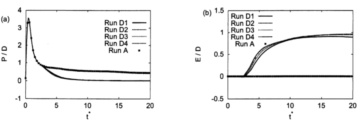
Figure 2: Comparison of the temporal evolutions of (a) the mean enstrophy produc-tion rate (S) dividedby the

mean

enstrophy dissipation rate (D) and of (b) the

mean

enstrophy production/inhibition rate due to polymer additives (P) divided by the mean enstrophy dissipation rate for Runs Dl,D2,$D3$, and D4. Run A is due to the

one-way coupling

case.

Because the kinetic energy decays with time, the Reynolds number

$R_{\lambda}(t)=\sqrt{\frac{20}{3\nu_{s}\epsilon(t)}}E(t)$, (10)

where $\epsilon(t)=v_{s}\langle(\nabla u)^{2}\rangle_{V}$is the mean dissipationrate of the kineticenergy, also decays with

time [12]. Thetypicalvalues of$R_{\lambda}(t)$ at$t^{*}=20$ are listed in table 1. Weclearly confirm that

$R_{\lambda}$ is order unity when $t^{*}=20$

.

In contrast, the local Weissenberg number _{$W_{i}(t)=\tau/\tau_{K}(t)$}

becomes larger than unity for all of the runs when $t^{*}=20$ as shown in table 1, and increase

with $\tau$. Thus at the end of simulationastate characterized by$R_{\lambda}=O(1)$ and $W_{i}\gg 1$, close

to the situation of elastic turbulence, is achieved. Wenote that the coil-stretch transitionof long-chain polymers

occurs

when $W_{i}=3-4[17].$

The enstrophy is defined by the mean squared vorticity

as

$E_{\omega}(t)=\langle\omega^{2}\rangle_{V}/2$ with $\omega=$

$\nabla\cross u$. The transport equation of$E_{\omega}(t)$ is derived from the $NS$ equations

as

$\frac{d}{dt}E_{\omega}(t) = \langle\omega\cdot(\omega\cdot\nabla u)\rangle_{V}+\langle(\nabla\cross\omega)\cdot(\nabla:T^{p})\rangle_{V}-v\langle(\nabla\omega)^{2}\rangle_{V}$ . (11)

The terms on the right hand side (R.H.S.) of Eq.(ll) are the mean enstrophy production,

mean

enstrophy exchanges due to polymers, and the

mean

enstrophy dissipation rate,

re-spectively $($named $P, E, and D in$ order). Figure2 shows the temporal evolutions of (a) the

mean

enstrophy production $(P)$ and of (b) the

mean

enstrophy exchanges due to polymers $(E)$, divided by the enstrophy dissipation rate $(D)$. These indicate that the contribution

of term $P$ to the production of enstrophy is almost negligible for $t^{*}>10$, while the term

$E$ shows the positive finite values in this range. This clearly represents the fact that the

vorticity stretching term has

an

negligible influence onproducing the turbulent fluctuations, and the turbulent state is kept by the term $E$ which is originated from the strong coupling

between the vorticity and stretching dumbbells. When

we

consider theNewtonian

case

(Run

A$)$, the term $P$ balances to the enstrophy dissipation,

so

that the vorticity stretching is the

(6)

$k|_{K}(t)$ $k|_{K}(t)$

Figure 3: Comparison of the kinetic energy spectra $E(k, t)$ by (a) normalized plot

of dissipation spectra using Kolmogorov scaling and by (b) compensated plot by multiplying $k^{a}$ obtained at $t^{*}=20$ for Runs Dl, D2, D3, and D4. Scaling exponent

$\alpha$ fOr eaCh

run

$S$i$S$ evaluated by the leaSt Square fitting in lhe range $2\leq$ 雇$K$$($オ$)$ $\leq 5$

decay of polymer solution turbulent flow is maintained due to the stronger elasticity which

is originated from the elastic energy restored in the decay regime of turbulence $(t^{*}<10)$

.

Figures 1 and 2 suggest that the mechanism of turbulence decay for polymer laden flow is quite different from the

case

of turbulence for Newtonian fluid. Decaying process of

turbulence is categorized into three stages

as

follows:

$s1)$ Turbulence develops from its initial value at the time that the

mean

energydissipation

reaches its maximum value. Then the dumbbells are rapidly stretched by turbulence, increasing $U(t)$

.

$s2)$ Turbulencestarts to decay by theactions ofviscosity andenergy transfer to the

ensem-ble ofdumbbells, while the dumbbells remain stretching up to the time $E(t)\sim U(t)$.

$s3)$ The restored potential energy $U(t)$ decays with time with the rate slower than $E(t)$,

meaningthat the back transfer ofenergyfrom the ensemble of dumbbells to turbulence

occurs.

In the stage$s1$) theenergy transfer fromturbulence to ensemble ofdumbbellsis active, while

the flow field is maintained by the back energy transfer from the ensemble of dumbbells in the stage $s3$). The turbulence statistics in stage $s3$) is thus governed by the elastic nature

of polymers, meaning that the situation is quite similar to the

case

of elastic turbulence. Next we investigate the scaling behavior of kinetic energy spectrum $E(k, t)$ obtained at $t^{*}=20$

.

The spectrum $E(k, t)$ is defined by

$E(k, t)=2\pi k^{2}\langle|\hat{u}(k, t)|^{2}\rangle_{s}$ (12)

in terms of the Fourier amplitude$\hat{u}(k, t)$ where $\langle\cdots\rangle_{s}$ is the average taken

over

the spherical

shell within $k-\triangle k/2<|k|\leq k+\triangle k/2$ in the wavenumber space. Figure 3 (a) compares

the kinetic energy spectra obtained for all of the runs, where we plotthe dimensionless form

ofdissipation spectra $\hat{D}(kl_{K}(t), t)$ defined using the Kolmogorov scaling

as

(7)

$10^{rightarrow 1}$ $10^{0}$ $10^{1}$

$k|_{K}(t)$

$10^{-1}$ $10^{0}$

$k|_{K}(t)$

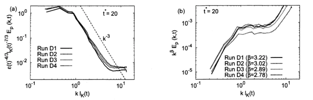
Figure 4: Comparison of the pressure spectra for (a) normalized plot using the

Kol-mogorov scaling obtained at $t^{*}=20$ and for (b) the compensated plot by

multiply-ing the factor $k^{\alpha}$, in which $\alpha$ is evaluated by the least square fitting in the range $2\leq kl_{K}(t)\leq 5.$

to stress the behavior in the range $kl_{K}(t)>1$. As shown in figure 3 (a), the normalized

spectra almost collapse in the range $kl_{K}(t)<1$, and they show the power-law decay for

$kl_{K}(t)>1$. The spectrumbecomes less steep and approaches to $k^{-2}$ with an increase of$W_{i},$

meaning that $E(k, t)$ is close to $E(k)\sim k^{-4}$

.

To see this point in more detail, we investigate

the compensated spectra $k^{\alpha}E(k, t)$ plotted infigure3 (b), where the exponent $\alpha$ is evaluated

bythe least square fit in the range$2\leq kl_{K}(t)\leq 5$

.

This figure clearly indicates that 1) there

is a clearscaling range for each curves of$W_{i},$ $2$) the value of$\alpha$ decreases with an increase of

$W_{i}$

.

The largest $W_{i}$ case shows $\alpha=4.14$ which isnear the values of3.5 and 3.8 obtained by

the elastic turbulence [1, 6, 7].

The power-law form of $E(k, t)$ observed in figure 3 implies that the pressure spectrum

$E_{p}(k, t)$ also obeys the power-law form. The pressure field$p(x, t)$ is determined by the $NS$

equations with

an

incompressible condition

as

$p(x, t)=\triangle^{-1}(-\nabla\cdot(u\cdot\nabla u)+\nabla\cdot(\nabla:T^{p}))$ . (14)

When the turbulence adequately decays while the dumbbells remain the fully stretched configurations, the first term of the R.H.S. ofEq.(14) is sufficientlysmallerthan the second one, leading to the relationship $p(x, t)\simeq\triangle^{-1}\nabla\cdot(\nabla : T^{p})$ for $W_{i}\gg 1[9]$. Thus the

statistics of pressure field is dominated by that of the polymer stress field. Figure 4 shows the comparison of the pressure spectra $E_{p}(k, t)=2\pi k^{2}\langle|\hat{p}(k, t)|^{2}\rangle_{s}$ obtained at $t^{*}=20$ for

all of the

runs.

The normalized plot by using the Kolmogorov scaling, shown in figure 4

(a), clearly represents that the pressure spectraobey the power-law form close to $k^{-3}$ in the

range $kl_{K}(t)>1$

.

This is almost consistent with the experimental result by [9]. Spectra

become less steep with

an

increase of $W_{i}$

.

This is confirmed by figure 4 (b) representing

the compensated plot $k^{\beta}E_{p}(k, t)$ where the exponent $\beta$ is also evaluated by the least

square

fitting in the range same as $E(k, t)$. We confirm the existence of plateaus in figure 4 (b)

although there are some scatter of data when compared to the case of $k^{\alpha}E(k, t)$ (figure 3

$(b))$. Thevalue of$\beta$ decreases with

an

increase of$W_{i}$, where$\beta=3.22,3.02,2.89$, and2.78 for

Runs Dl,D2,$D3$, and D4. This feature is similar to the case for the kinetic energy spectrum

(8)

$(z-<z>)/0_{z}$ $(z-<z>)/\sigma_{z}$

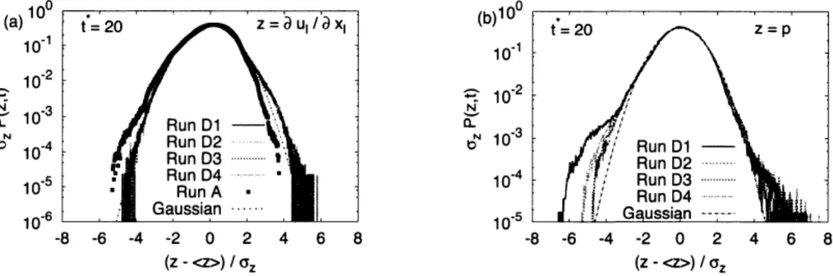
Figure 5: Comparison of the normalized PDFs for (a) longitudinal velocity derivative

$\partial_{L}u_{L}$ and for (b) pressure

$p$ obtained at $t^{*}=20$ for Runs Dl, D2, D3 and D4.

Similarities ofpower-law spectra ofboth $E(k)$ and $E_{p}(k)$ between the present numerical

results and the results by experimental observation suggest that the one-point statistics

of the velocity derivative and pressure fields may show the strong non-Gaussianity [8, 9]. We further investigate the PDF behaviors for both the longitudinal velocity derivativefield

$\partial_{L}u_{L}(x, t)$ and the pressure field$p(x, t)$. Figure 5 shows the resulting

curves

obtained by the

data at $t^{*}=20$for (a) $\partial_{L}u_{L}(x, t)$ and (b) $p(x, t)$, where we compare thecurves made by the

standardized plot. Weconfirm that the PDF formisalmostinsensitive tothevariationof$W_{i}$

for both cases, and slightlydeviatesfrom the Gaussian for $\partial_{L}u_{L}$

.

The PDF form of$\partial_{L}u_{L}$ by

Runs $DI$-D4 becomes almost symmetric, meaning that the skewness factor of $\partial_{L}u_{L}$, which

is related to the

mean

vorticity production in isotropic turbulence, is almost

zero.

This is in sharp contrast tothe one-way coupling

case

(Run A), and is alsoconsistent with the results of figure 2. While the curves for $p(x, t)$ show almost Gaussian although the each

curves

are

slightly skewed. Thus the velocity gradient and pressure field statistics manifest the less

intermittent fluctuations than those by experimental results [8, 9], and

are

approximately

Gaussian form. This suggests that the mechanism for producing thenon-Gaussian statistics

in experimentsmaynot beattributed to the effectsof polymers, perhaps is due to the nature

oflarge-scale properties like the forcing mechanism. This calls further studies in the

case

for steady flow by introducing appropriate forcing mechanism. Also the PDF tail behavior is sensitiveto the resolution condition [18],

so

that

we

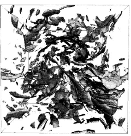
mayneed further increaseofspatialgrid points to clarify the discrepancy between the present numerical and previous experimental results.

We discuss the power-law form of thespectraobtained in this study. Figure3 (b) suggests thatthe scaling exponent $\alpha$for the kinetic energyspectrum approachesto the value of4when

$W_{i}$ is increased further. The spectral form $E(k)\sim k^{-4}$ reminds

us

that of two-dimensional

turbulence in the enstrophy inertial

range,

suggested by Saffman [19]. The key idea is the

formation of the thin layer ofvorticityfield and leading to the largejump ofvorticity, yields

the power-law spectrum of vorticity spectrum $E_{\omega}(k)\sim k^{-2}$. Thus $E(k)\sim k^{-2}E_{\omega}(k)\sim k^{-4}.$

This raises the question of how the field structure of vorticity field is characterized when

$W_{i}\gg 1$. We expect to observe the large jump of vorticity, i.e. the regions having larger

$|\nabla\omega|$ localize in space. Figure 6 shows the iso-surface of $|\nabla\overline{\omega}|$ obtained by Run D4 with

(9)

Figure6: Visualization of iso-surface of the absolute ofvorticity derivative field $|\nabla\overline{\omega}|$

obtained at $t^{*}=20$ of Run D4.

the zig-zag fluctuations

on

the objects. This figure indicates that $|\nabla\overline{\omega}|$ localizes in space as

thesheet-like structures. This

seems

to support the idea bySaffman [19], although

we

donot know why such a sheet-like structure is formed due to the effect ofpolymers. Moreover we

need further examinations by performing the simulations with larger $W_{i}$ values than those

by present study to confirm the asymptotic value of$\alpha$ when $W_{i}arrow\infty.$

Finally we comment on the relationship between $E(k)$ and $E_{p}(k)$. In the final period of

decay, the elastic energy for the ensemble of dumbbells is larger than the kinetic energy of fluid motion, as shown in figure 1. Also the mean enstrophy is produced by the polymer stress field rather than the vorticity stretching term originated from the advection term in the $NS$ equations. These facts yield the evaluation of the order of velocity _$u$ _{and pressure}

$p$

as

$|u|\sim(\nu/l)|T^{p}|,$ $l$ being the characteristic scale in the scaling range, and

$p\sim|T^{p}|$

from Eq.(14) with $W_{i}\gg 1$. This estimation leads to the relationship $E(k)\sim(\nu k)^{-2}E_{p}(k)$,

so that we have $\alpha-\beta=2$. On the other hand, the numerical results by figures 3 and 4

indicate$\alpha-\beta=1.38,1.29,1.30$, and 1.36 for Runs Dl,D2,$D3$, and D4, being smaller than 2,

although the values of$\alpha-\beta$ are insensitiveto the variation of$W_{i}$. This

means

that thesimple

dimensional evaluation does not work well. We have no ideato explain this discrepancy at present, but this analysissuggests that the values of scaling exponent $\alpha$ and$\beta$

are

not simply

extracted from the arguments by the dimensional grounds.

In summary, we investigated the scaling behavior of both the kinetic energy and pressure

spectrum in decaying isotropic turbulence with polymer additives for various values of $W_{i}$

for $W_{i}\gg 1$. We obtained the power-law forms of $E(k)\sim k^{-\alpha}$ and $E_{p}(k)\sim k^{-\beta}$ in the

range $kl_{K}>1$ when turbulence adequately decayed and the elastic energy became _larger

than the kinetic energy offluid motions. Exponents $\alpha$ and $\beta$ were approximately 4.2–4.6

and 2.8–3.2, and decreased with the increase in $W_{i}$. The value of $\beta$

was

similar to the

values obtained in the recent experimental study of elastic turbulence $(\beta=3)$, while the

value of $\alpha$ obtained by the largest value of $W_{i}$ was slightly larger than those obtained by

experiments $(\alpha=3.5)[1]$ and by the DNS ofthe constitutive equations $(\alpha=3.8)[6,7])$.

Significant difference is observed in the PDF behavior of velocity derivative and pressure

fields, where

we

observed the behavior close to the Gaussian irrespective of$W_{i}$, in contrast

to the non-Gaussian statistics by experimental results [8, 9].

T. W. and T. G. were supported in part by Grants-in-Aid for Scientific Research Nos.

(10)

Sci-ence, and Technology of Japan. T. W. would like to thank

S.

Uno and D. Sugimoto for

their assistance in writingthe parallelized code. The authors would liketothank the Theory and Computer Simulation Center of the National Institute for Fusion Science and JHPCN

and HPC at the Information Technology Center of Nagoya University for providing the computational

resources.

References

[1] A. Groisman and V. Steinberg, Nature 405, 53-55, (2000) [2] A.

Groisman

and V. Steinberg, Nature 410, 905-908, (2001)

[3] T. Burghelea, E. Segre, and V. Steinberg, Phys. Rev. Lett. 92, 164501 (2004).

[4] P. E. Arratia, C. C. Thomas, J. Diorio, and J. P. Gollub, Phys. Rev. Lett. 96, 144502

(2006).

[5] T. Burghelea, E. Segre, and V. Steinberg, Phys. Rev. Lett. 96, 214502 (2006).

[6] S. Berti, A. Bistagnino, G. Boffetta, A. Celani and S. Musacchio, Phys. Rev. $E77,$

055306 (2008).

[7] S. Berti and G. Boffetta, Phys. Rev. $E82$, 036314 (2010).

[8] A. Groisman and V. Steinberg, New J. Phys., 6, 29 (2004).

[9] Y. Jun and V. Steinberg, Phys. Rev. Lett. 102, 124503 (2009). [10] T. Watanabe and T. Gotoh, J. Fluid. Mech. 717, 535 (2013). [11] A. Fouxon and V. Lebedev, Phys. Fluids 15, 2060 (2003).

[12] T. Watanabe and T. Gotoh, accepted for publication in J. Phys.: