Generalized integrable evolution equations with an infinite number of free parameters (Workshop on Nonlinear Water Waves)

全文

(1)33 Generalized integrable evolution equations with an infinite number of free parameters Nail Akhmedievl, Adrian Ankiewicz1, Shalva Amiranashvili2 and Uwe Bandelow2 1 Optical Sciences Group, Research School of Physics and Engineering, The Australian National University, Canberra, ACT 2600, Australia. 2 Weierstrass Institute for Applied Analysis and Stochastics, Mohrenstrasse 39, 10117 Berlin, Germany. Evolution equations such as the nonlinear Schrödinger equation (NLSE) can be extended to include an infinite number of free parameters. The extensions are not. unique. We give two examples that contain the NLSE as the lowest‐order PDE of each set. Such representations provide the advantage of modelling a larger variety of physical problems due to the presence of an infinite number of higher‐order terms. in this equation with an infinite number of arbitrary parameters. An example of a rogue wave solution for one of these cases is presented, demonstrating the power of the technique.. I.. INTRODUCTION. The mathematical description of physical processes is a crucial step towards our ability to. understand nature. A time derivative in this description provides the possibility of relating the past and the future of the evolution. In other words, equations with time derivatives allow. us to predict future dynamics based on the present conditions. These are known as evolution. equations. A few of them are integrable in the sense that their solutions can be written analytically. Finding new integrable equations leads to further progress in describing nature. Well‐known examples of evolution equations are the KdV[1] , the nonlinear Schrödinger. equation (NLSE) [2] and some of its extensions [3]. The NLSE is one of the basic models of nonlinear wave propagation in optical fibers [4], water waves [5, 6] and generally in nonlinear. dispersive media [7, 8]. This equation and its variations have been instrumental in describing phenomena of temporal and spatial soliton propagation [8], their interactions [9], modulation. instability [10], periodic and localized breathers [11−15], supercontinuum generation [16],.

(2) 34 Fermi‐Pasta‐Ulam Recurrence [17], Bose‐Einstein condensates [18] and rogue waves [19−21]. However, in order to increase the accuracy of modelling, the NLSE has to be extended. to include additional terms [22] that are responsible for higher‐order dispersion [23] and nonlinear effects such as self‐steepening and self‐frequency shift [24, 25]. These terms are. important in the description of higher‐amplitude waves [26, 27] and shorter duration pulses [28]. Very often, on extending the equations, while we gain in accuracy, we lose in integrability of the NLSE. Fortunately, integrability can be restored for special choices of the coefficients. in the higher‐order terms. For extensions including third order terms, the choice of the. coefficients that admit integrability are well‐known. These cases include the Hirota [29] and. Sasa‐Satsuma (SSE) [30] equations. However, the next step of such extensions is still not completely classified. For the branch of extensions that includes the Hirota equation, certain. higher‐order evolution equations are known. These include the fourth‐order Lakshmanan‐. Porsezian‐Daniel (LPD) equation [31] and a fifth‐order equation [32]. Moreover, the whole infinite extension and its soliton and rogue wave solutions can be presented explicitly [33, 34]. An important step is that the whole set can be written in the form of one ‘general. equation’ [33, 34]. Moreover, this general equation can have an infinite number of operators controlling time evolution of a system [33, 34]. It includes known equations as particular cases with arbitrary real coefficients which govern the contribution of each operator to the. whole set.. The power of such representation lies in the variability of these coefficients.. When all of them are zero except one, we obtain a particular case. Having two or more coefficients being nonzero provides more complicated equations that can be of interest due. to the special case in physics that such an equation may describe.. One example is the. Heisenberg spin chain dynamics [43]. Such ‘general equations’ could be of great importance for physics because higher‐order terms in this equation may describe finer effects such as. higher‐order dispersion or higher‐order nonlinearities in the wave propagation phenomena. They improve the accuracy of the basic approximation that is usually described by the lowest‐order equation.. Unfortunately, not all higher‐order terms in these generalizations result in integrable equations. A specific set of coefficients is required for these integrable cases. It is indeed fortunate when such an ‘upgrade’ belongs to an integrable case. The chances are low if there is only one case that starts with the given base equation.. Finding new equations.

(3) 35 is thus an important task which may significantly improve the accuracy of modelling of physical phenomena. We have found that there are at least two ‘general equations’ that. have the NLSE as a base. One of them is a ‘generalized Hirota equation’ [33, 34], while the other one, found more recently [35], is a ‘generalized Sasa‐Satsuma equation’. Both start with the NLSE as a base evolution equation. Thus, both of them could be called NLSE. sets. In order to avoid confusion and distinguish them explicitly, we label them here as the generalized Hirota and generalized Sasa‐Satsuma equations. The first few equations of. the Hirota extension are the NLSE [8], the third‐order Hirota equation [29], fourth‐order LPD equation [31] and the quintic equation of this sequence [32, 36]. Higher‐order infinite extensions of this set have been presented in explicit forms in [33, 34]. On the other hand, the generalised Sasa‐Satsuma equation has, as the starting equations, the NLSE and the. third‐order Sasa‐Satsuma equation [30, 37, 38]. Higher‐order infinite extensions have been discovered in our recent work [35]. In the present work, we review the progress made towards the infinite extention of the NLSE with the addition of an infinite number of higher‐order terms.. These terms keep. each of the considered general equations integrable, while at the same time allowing us to include an infinite number of free parameters that control these higher‐order terms. The latter provides infinitely many degrees of freedom in describing physical models but keeps the whole equation integrable. This has both advantages and disadvantages. The advantage. is that solutions can be presented in analytical form. The disadvantage is that integrability still restricts the modelling and keeps it in a rigid frame. However, we believe that, on finding more such general equations, the frame can be significantly widened.. II.. GENERALIZED HIROTA EQUATION. The technique of extending the NLSE has been developed in [33, 34]. Below, we present only the final results. Namely, the generalised Hirota equation can be written in the form:. i\psi_{t}+\alpha_{2}K_{2}[\psi(x, t)]-i\alpha_{3}K_{3}[\psi(x, t)] +\alpha_{4}K_{4}[\psi(x, t)]-i\alpha_{5}K_{5}[\psi(x, t)] +\alpha_{6}K_{6}[\psi(x, t)]-i\alpha_{7}K_{7}[\psi(x, t)] +\alpha_{8}K_{8}[\psi(x, t)]- =0,. (1).

(4) 36 where t is the evolution variable,. x. is the transverse variable, while each functional K_{j}[\psi(x, t)]. represents a particular operator of order j . Coefficients \alpha_{j} are arbitrary real parameters. Importantly, they do not have to be small. This freedom allows us to go well beyond the simple extension of the NLSE with corrective perturbative terms.. In the lowest, second order, we obtain the fundamental nonlinear Schrödinger equation:. i\psi_{t}+\alpha_{2}K_{2}[\psi(x, t)]=i\psi_{t}+\alpha_{2}(\psi_{xx}+ 2|\psi|^{2}\psi)=0 . Taking. \alpha_{2}=\frac{1}{2}. (2). or rescaling the t ‐variable, we get the NLSE in standard form. By adding. the third order operator, K_{3} , we obtain the Hirota equation [29, 39]:. i\psi_{t}+\alpha_{2}(\psi_{xx}+2|\psi|^{2}\psi)-i\alpha_{3}(\psi_{xxx}+6|\psi|^ {2}\psi_{x})=0 .. (3). Now, as a particular case of Eq.(3), we can take \alpha_{2}=0 . The resulting equation. \psi_{t}-\alpha_{3}(\psi_{xxx}+6|\psi|^{2}\psi_{x})=0 ,. (4). is known as the ‘basic’ Hirota equation or as the ‘complexified’ modified Korteweg de Vries. (mKdV) equation [40]. Taking. \alpha_{3}=. −lleads to its standard form. The common factor i is. canceled when transforming (3) into Eq.(4). This cancellation can be done for all equations (1) when the coefficients with even indices are zero, i.e. \alpha_{2n}=0 . However, solutions of these equations can be sought in either complex or real forms. For example, when the function \psi. is real (and \alpha_{3}=1 ), Eq.(4) becomes the real. mKdV :. \psi_{t}-\psi_{xxx}+6\psi^{2}\psi_{x}=0 .. (5). Solutions of the real mKdV equation are related to the solutions of the Korteweg de Vries. (KdV) equation through the Miura transformation [41]. Eq.(5) has rational solutions [42] that also have a single high peak that can be viewed as a rogue wave at the center. How‐ ever, these elevated peaks are not completely localized, but are positioned on soliton‐like. structures [42]. With the fourth order operator, K_{4},. K_{4}[\psi(x, t)]=\psi_{xxxx}+8|\psi|^{2}\psi_{xx}+6|\psi|^{4}\psi+4|\psi_{x}|^ {2}\psi+6\psi_{x}^{2}\psi^{*}+2\psi^{2}\psi_{xx}^{*} .. (6). the equation is known as the LPD [43−45] equation. Further, the fifth order operator, K_{5} is given by:. K_{5}[\psi(x, t)]=\psi_{xxxxx}+10|\psi|^{2}\psi_{xxx}+10(|\psi_{x}|^{2}\psi) _{x}+20\psi^{*}\psi_{x}\psi_{xx}+30|\psi|^{4}\psi_{x} .. (7).

(5) 37 Even from this brief analysis, we can see the wide range of possibilities that the general. equation (1) provides. It includes many particular cases and it allows us to combine them into a unified model. Moreover, the original NLSE does not have to be part of it (we can have \alpha_{2}=0 ), but it helps to suggest the form of some solutions. Further, the sixth order operator, K_{6} , first found in [34], has the following explicit form:. K_{6}[\psi(x, t)]=\psi_{xxxxxx}+\psi^{2}[60|\psi_{x}|^{2}\psi^{*}+50(\psi^{*})^ {2}\psi_{xx}+2\psi_{xxxx}^{*}]. (8). +\psi[12\psi^{*}\psi_{xxxx}+8\psi_{x}\psi_{xxx}^{*}+22|\psi_{xx}|^{2}+ 18\psi_{xxx}\psi_{x}^{*}+70(\psi^{*})^{2}\psi_{x}^{2}]+20(\psi_{x})^{2}\psi_{xx} ^{*}. +10\psi_{x}[5\psi_{xx}\psi_{x}^{*}+3\psi^{*}\psi_{xxx}]+20\psi^{*}\psi_{xx}^{2} +10\psi^{3}[(\psi_{x}^{*})^{2}+2\psi^{*}\psi_{xx}^{*}]+20|\psi|^{6}\psi. while the seventh order operator, K_{7} , is:. K_{7}[\psi(x, t)]=\psi_{xxxxxxx}+70\psi_{xx}^{2}\psi_{x}^{*}+112|\psi_{xx}|^{2} \psi_{x}+98|\psi_{x}|^{2}\psi_{xxx}. (9). +70\psi^{2}[\psi_{x}[(\psi_{x}^{*})^{2}+2\psi^{*}\psi_{xx}^{*}]+\psi^{*}(2\psi_ {xx}\psi_{x}^{*}+\psi_{xxx}\psi^{*})]+28\psi_{x}^{2}\psi_{xxx}^{*} +14\psi[\psi^{*}(20|\psi_{x}|^{2}\psi_{x}+\psi_{xxxxx})+3\psi_{xxx}\psi_{xx} ^{*}+2\psi_{xx}\psi_{xxx}^{*}+2\psi_{xxxx}\psi_{x}^{*} +\psi_{x}\psi_{xxxx}^{*}+20\psi_{x}\psi_{xx}(\psi^{*})^{2}]+140|\psi|^{6} \psi_{x}+70\psi_{x}^{3}(\psi^{*})^{2} +14\psi^{*}(5\psi_{xx}\psi_{xxx}+3\psi_{x}\psi_{xxxx}). .. The highest operator that we give here is K_{8} :. K_{8}[\psi(x, t)]=\psi_{xxxxxxxx}. (10). +14\psi^{3}[40|\psi_{x}|^{2}(\psi^{*})^{2}+20\psi_{xx}(\psi^{*})^{3}+ 2\psi_{xxxx}^{*}\psi^{*}+3(\psi_{xx}^{*})^{2}+4\psi_{x}^{*}\psi_{xxx}^{*}] +\psi^{2}[28\psi^{*}(14|\psi_{xx}|^{2}+11\psi_{xxx}\psi_{x}^{*}+6\psi_{x} \psi_{xxx}^{*})+238\psi_{xx}(\psi_{x}^{*})^{2}+336|\psi_{x}|^{2}\psi_{xx}^{*} +560\psi_{x}^{2}(\psi^{*})^{3}+98\psi_{xxxx}(\psi^{*})^{2}+2\psi_{xxxxxx}^{*}]+ 2\psi\{21\psi_{x}^{2}[9(\psi_{x}^{*})^{2}+14\psi^{*}\psi_{xx}^{*}] +\psi_{x}[728\psi_{xx}\psi_{x}^{*}\psi^{*}+238\psi_{xxx}(\psi^{*})^{2}+ 6\psi_{xxxxx}^{*}]+34|\psi_{xxx}|^{2}+36\psi_{xxxx}\psi_{xx}^{*}. +22\psi_{xx}\psi_{xxxx}^{*}+20\psi_{xxxxx}\psi_{x}^{*}+161\psi_{xx}^{2} (\psi^{*})^{2}+8\psi_{xxxxxx}\psi^{*}\}+182\psi_{xx}|\psi_{xx}|^{2} +308\psi_{xx}\psi_{xxx}\psi_{x}^{*}+252\psi_{x}\psi_{xxx}\psi_{xx}^{*}+196\psi_ {x}\psi_{xx}\psi_{xxx}^{*}+168|\psi_{x}|^{2}\psi_{xxxx}. +42\psi_{x}^{2}\psi_{xxxx}^{*}+14\psi^{*}(30\psi_{x}^{3}\psi_{x}^{*}+ 4\psi_{xxxxx}\psi_{x}+5\psi_{xxx}^{2}+8\psi_{xx}\psi_{xxxx}). +490\psi_{x}^{2}\psi_{xx}(\psi^{*})^{2}+140\psi^{4}\psi^{*}[(\psi_{x}^{*})^{2}+ \psi^{*}\psi_{xx}^{*}]+70|\psi|^{8}\psi. The general equation can be continued up to infinity. The complexity of the operators K_{j}. grows with the order j . The general iterative rules for obtaining these operators are given in.

(6) 38 [33, 34]. The equation when the two coefficients. \alpha_{3}. and. \alpha_{4}. are arbitrary has been considered. earlier in [46, 47]. In particular, soliton solutions of this equation were given in [46], while rogue wave solutions were presented in [47]. The generalised Hirota equation (1) has been derived for the case of. 2\cross 2. matrix Lax pairs. Therefore, the Sasa‐Satsuma equation which. requires the Lax pairs to be based on. III.. 3\cross 3. matrices is not part of this set.. GENERALIZED SASA‐SATSUMA EQUATION. We write the generalized Sasa‐Satsuma equation in the same form as Eq.(l):. i\psi_{t}+\alpha_{2}S_{2}[\psi(x, t)]-i\alpha_{3}S_{3}[\psi(x, t)]. (11). +\alpha_{4}S_{4}[\psi(x, t)]-i\alpha_{5}S_{5}[\psi(x, t)] +\alpha_{6}S_{6}[\psi(x, t)]-i\alpha_{7}S_{7}[\psi(x, t)] +\alpha_{8}S_{8}[\psi(x, t)]- =0. However, we have chosen different notations for the functionals S_{j}[\psi(x, t)] as they are indeed. different from K_{j}[\psi(x, t)] . As above, transverse variable.. Coefficients. \alpha_{j}. t. here is the evolution variable (time) while. x. is the. are again arbitrary real numbers making Eq.(l) an. infinitely variable integrable evolution equation for a variety of applications that describe soliton and rogue wave phenomena.. The lowest order functional S_{2}[\psi(x, t)] in Eq.(1) is given by. S_{2}[\psi(x, t)]=\psi_{xx}+4|\psi|^{2}\psi . Thus, when all. \alpha_{j}. are zero except for the. \alpha_{2}. (12). , Eq. (1) is simply the NLSE but differently. normalised from (1) for compatibility with other functionals in the equation. The third order functional. S_{3}[\psi(x, t)]. is. S_{3}[\psi(x, t)]=\psi_{xxx}+3(|\psi|^{2})_{x}\psi+6|\psi|^{2}\psi_{x} . Therefore, when,. \alpha_{3}. (13). is nonzero and \alpha_{2}=1/2 , we have the SSE:. i \psi_{t}+\frac{\psi_{xx}}{2}+2|\psi|^{2}\psi=i\alpha_{3}[\psi_{xxx}+3(|\psi|^ {2})_{x}\psi+6|\psi|^{2}\psi_{x}] .. (14). The fourth‐order operator,. S_{4}[\psi(x, t)]=\psi_{xxxx}+6\psi_{xx}^{*}\psi^{2}+24|\psi|^{4}\psi+ 12|\psi_{x}|^{2}\psi+14|\psi|^{2}\psi_{xx}+8\psi^{*}\psi_{x}^{2} ,. (15).

(7) 39 while the next one is. S_{5}[\psi(x, t)]=\psi_{xxxxx}+80|\psi|^{4}\psi_{x}+5\psi^{2}\psi_{xxx}^{*}+ 25\psi(|\psi_{x}|^{2})_{x}. (16). +40|\psi|^{2}\psi^{2}\psi_{x}^{*}+20|\psi_{x}|^{2}\psi_{x}+15|\psi|^{2} \psi_{xxx}+30\psi^{*}\psi_{x}\psi_{xx}. At the next level,. S_{6}[\psi(x, t)]=\psi_{xxxxxx}+55\psi^{3}(\psi_{x}^{*})^{2}+45\psi_{x}^{2} \psi_{xx}^{*}+32\psi\psi_{x}\psi_{xxx}^{*}+43\psi^{*}\psi_{x}\psi_{xxx}. (17). +37\psi\psi_{x}^{*}\psi_{xxx}+175|\psi|^{2}\psi^{*}\psi_{x}^{2}+53|\psi_{xx} |^{2}\psi+31\psi^{*}\psi_{xx}^{2}+20|\psi|^{2}\psi_{xxxx}. +160|\psi|^{6}\psi+110\psi^{*}\psi^{3}\psi_{xx}^{*}+330|\psi\psi_{x}|^{2}\psi+ 170|\psi|^{4}\psi_{xx}+8\psi^{2}\psi_{xxxx}^{*}+95|\psi_{x}|^{2}\psi_{xx}. The expressions for S_{7}[\psi(x, t)] and higher are too cumbersome to be given here, but our. technique, presented in [35] is straightforward, allowing one to write them explicitly for any order j . We stress that the expressions for S_{j}[\psi(x, t)] are different from K_{j}[\psi(x, t)] given in the previous section. The reason is that the Lax pairs for these equations involve. matrices rather than. 2\cross 2. 3\cross 3. for the Hirota branch. As a result, the solutions of Eq.(11). are significantly more involved than the solutions of Eq.(l). Such complexity starts right from the lowest order Eq.(11) which is the SSE [30, 37, 38, 48−51]. Both soliton solutions [37, 48, 49] and rogue wave solutions [52] have much more complicated structures than the corresponding solutions for the NLSE or Hirota equations. They involve more parameters in the solutions and thus allow us to describe more complicated profiles. In particular, the. basic SSE has single‐soliton solutions that have no analogs in the NLSE case. In addition. to the common bell‐shaped solitons, it has soliton solutions with two maxima [30] and even with multiple maxima [49]. Moreover, the SSE has soliton solutions with complex oscillating patterns in the (x, t) ‐plane [48]. Solutions become even more complicated when they contain a background in the form of a plane wave [50]. The complexities tend to accumulate when dealing with the higher‐order equations of the generalized SSE. Due to this complexity, even. for the basic SSE, only first‐order solutions have been derived so far [35].. IV.. SIMPLE EXAMPLE OF EXACT SOLUTION OF THE GENERALIZED. HIROTA EQUATION (1) The power of the generalized equation approach can be demonstrated by the fact that. we can seek solutions of Eq.(l) or Eq.(11) in a general form, taking into account the whole.

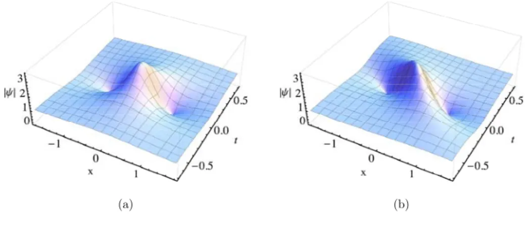
(8) 40 infinite set of operators involved in the equation. For illustrative purposes, we will demon‐. strate this only for Eq.(l). Namely, the first‐order rogue wave solutions for Eq.(l) can be written in explicit form [47]:. \psi(x, t)=c[4\frac{1+2iB_{r}t}{D(x,t)}-1]e^{i\phi_{r}t} , where. c. (18). is an arbitrary background while. B_{r}= \sum_{n=1}^{\infty}\frac{n(2n)!}{(n!)^{2} \alpha_{2n^{C^{2n} =2c^{2} (\alpha_{2}+6c^{2}\alpha_{4}+30c^{4}\alpha_{6}+140c^{6}\alpha_{8}+630c^{8} \alpha_{10}+\cdots). ,. (19). and. D(x, t)=1+4B_{r}^{2}t^{2}+4(cx+v_{r}t)^{2} ,. (20). where. v_{r}= \sum_{n=1}^{\infty}\frac{(2n+1)!}{(n!)^{2} \alpha_{2n+1^{C^{2n+1}. (21). =2c^{3}(3\alpha_{3}+15c^{2}\alpha_{5}+70c^{4}\alpha_{7}+315c^{6}\alpha_{9}+ 1386c^{8}\alpha_{11}+\cdots). .. The coefficient \phi_{r} in the exponential factor of (18) is given by:. \phi_{r}=c^{2}\sum_{n=1}^{\infty}\frac{(2n)!}{(n!)^{2} \alpha_{2n^{C^{2n-2}. (22). =2c^{2}(\alpha_{2}+3c^{2}\alpha_{4}+10c^{4}\alpha_{6}+35c^{6}\alpha_{8}+ 126c^{8}\alpha_{10}+\cdots) The tilt factor of odd‐order,. v_{r}. .. (or “velocity”) in (21) depends only on the coefficients of the operators. \alpha_{2n+1} ,. while the exponential factor, \phi_{r} , and the stretching factor, B_{r} , depend. only on the coefficients of the even‐order operators. \alpha_{2n} .. These observations allow us to make. some general conclusions about the rogue wave profiles. Two illustrative examples are shown in Fig.1. We can see from this figure that the tilt appears only when. \alpha_{5}. is non‐zero. Here,. due to limited space, we restrict ourselves with these two illustrations only. More solutions. presented in [36, 53] show some unexpected features.. V.. CONCLUSIONS. A generalized integrable equation with infinite number of free parameters is a novel approach in the theory of integrable equations. The two equations considered here include,.

(9) 41 41 as particular cases, known equations such as NLSE, Hirota equation, Sasa‐Satsuma equation, mKdV, etc. However, in combination with higher‐order terms in the general equation, they. become a powerful tool for modelling a wider range of physical problems.. |\psi. 1\psi. (a). FIG. 1: Rogue waves of Eq.(18), when c=1,. (b). ( a)\alpha_{4}=\frac{1}{4} and (b) \alpha_{4}=1/4, \alpha_{5}=\frac{1}{16} . All other. \alpha_{j} ’s in both cases are zero.. Each individual integrable evolution equation from either set is not just a special isolated case or a mathematical curiosity. NLSE extensions are usually considered to be improved. models for a more accurate description of nonlinear wave propagation in the ocean [27, 54, 55] and in optical fibers [23, 28]. Normally, these extensions are approximate, as they use small coefficients when dealing with higher‐order terms. The exactly integrable cases described. above are beyond these approximations. As such, they may expand the range of applicability of these models. Moreover, linear dispersion in our approaches can be modelled accurately. up to an infinite number of terms in the expansion. Although nonlinear terms become fixed. in this case, the deviations from realistic situation may be small. An additional advantage is that solutions can be analytically presented around the above integrable cases in approximate. forms, thus extending the range of their applicability.. Namely, perturbation techniques. based on these extended models may be a better solution [56] than choosing the NLSE as a ‘zero order’ approximation. Thus, adding new members to the family of integrable equations should be considered as adding significantly more power to our ability to do. accurate mathematical modelling of physical phenomena..

(10) 42 Acknowledgments. N.A. and A.A. acknowledge the support of the Australian Research Council (Discov‐. ery Project numbers DP140100265 and DP150102057). U.B. acknowledges support by the German Research Foundation in the framework of the Collaborative Research Center 787. Semiconductor Nanophotonics under project B5. Sh.A. acknowledges support of the German Research Foundation under Project 389251150.. [1] C. S. Gardner, J. M. Greene, M. D. Kruskal, R. M. Miura, Method for solving the Korteweg de Vries equation, Phys. Rev. Lett., 19, 1095—1097 (1967). [2] V. E. Zakharov and A. B. Shabat, Exact theory of two‐dimensional self‐focusing and one‐ dimensional self‐modulation of waves in nonlinear media, J. Exp. Theor. Phys., 34, 62 ‐ 69,. (1972). [3] N. Akhmediev and A. Ankiewicz, Solitons, nonlinear pulses and beams, (Chapman and Hall, London, 1997). [4] A. Hasegawa and F. Tappert, Transmission of stationary nonlinear optical pulses in dispersive dielectric fibers. I. Anomalous dispersion, Appl. Phys. Lett., 23, 142—144 (1973).. [5] V. E. Zakharov, Stability of periodic waves of finite amplitude on a surface of deep fluid, J. Appl. Mech. Tech. Phys., 9, 190—194 (1968). [6] Yuen H. C. & Lake, B. M. Nonlinear dynamics of deep‐water gravity waves. Adv. Appl. Mech. 22, 67‐228 (1982).. [7] Benney D. J. & Newell, A. C. The Propagation of Nonlinear Wave Envelopes. J. Math. Phys. 46, 133‐139 (1967).. [S] V. E. Zakharov and A. B. Shabat, Exact theory of two‐dimensional self‐focussing and one‐ dimensional self‐modulation of waves in nonlinear media, Sov. Phys. JETP, 34, 62 (1972). [9] V. S. Gerdjikov, I. M. Uzunov, E. G. Evstatiev, G. L. Diankov, Nonlinear Schrödinger equation and. N ‐soliton. interactions, Phys. Rev. E55 ,. 6039 (1997).. [10] N. Akhmediev and V. I. Korneev, Modulation instability and periodic solutions of the non‐ linear Schrödinger equation, Theor. Math. Phys. (USSR), 69, 1089 (1986). [Translated from Teor. Mat. Fiz., 69, 189‐ 194 (1986)]..

(11) 43 [11] N. Vishnu Priya, M. Senthilvelan, and M. Lakshmanan, ABs, Ma solitons, and general breathers from rogue waves: A case study in the Manakov system, Phys. Rev. E,. 88 ,. 022918. (2013). [12] V. A. Makarov, V. M. Petnikova, The distinctive feature of long time adiabatic modulation in the context of cnoidal wave and AB interaction, Laser Physics, 27, 025402 (2017). [13] F. Baronio, Akhmediev breathers and Peregrine solitary waves in a quadratic medium, Opt. Lett., 42, 1756 (2017).. [14] B. Kibler, J. Fatome, C. Finot, G. Millot, F. Dias, G. Genty, N. Akhmediev, J. M. Dudley, The Peregrine soliton in nonlinear fibre optics. Nature Phys. 6, 790 (2010). [15] F. Baronio, A. Degasperis, M. Conforti and S. Wabnitz, Solutions of the Vector Nonlinear Schrödinger Equations: Evidence for Deterministic Rogue Waves. Phys. Rev. Lett., 109,. 044102 (2012). [16] J. M. Dudley, G. Genty, and S. Coen, Supercontinuum generation in photonic crystal fiber, Rev. Mod. Phys. 78, 1135 (2006).. [17] A. Mussot, A. Kudlinski, M. Droques, P. Szriftgiser and N. Akhmediev, Fermi‐Pasta‐Ulam Recurrence in Nonlinear Fiber Optics: The Role of Reversible and Irreversible Losses, Phys.. Rev. X, 4, 011054 (2014). [18] V. B. Bobrov and S. A. Trigger, Bose‐Einstein condensate wave function and nonlinear Schrödinger equation, Bull. Lebedev Phys. Inst., 43, 266 (2016). [19] F. Baronio, M. Conforti, A. Degasperis and S. Lombardo, Rogue waves emerging from the resonant interaction of three waves, Phys. Rev. Lett., 111, 114101 (2013). [20] F. Baronio, A. Degasperis, M. Conforti, and S. Wabnitz, Solutions of the Vector Nonlinear Schrödinger Equations: Evidence for Deterministic Rogue Waves, Phys. Rev. Lett., 109,. 044102 (2012).. [21] N. Akhmediev, A. Ankiewicz and M. Taki, Waves that appear from nowhere and disappear without a trace, Phys. Lett. A 373, 675—678 (2009).. [22] Dysthe, K. B. Note on a modification to the nonlinear Schrödinger equation for application to deep water waves. Proc. R. Soc. Lond. A 369, 105—114 (1979). [23] S. B. Cavalcanti, J. C. Cressoni, H. R. da Cruz, and A. S. Gouveia‐Neto. Modulation insta‐ bility in the region of minimum group‐velocity dispersion of single‐mode optical fibers via an. extended nonlinear Schrödinger equation, Phys. Rev. A, 43,6162-6165 (1991)..

(12) 44 [24] M. Trippenbach and Y. B. Band, Effects of self‐steepening and self‐frequency shifting on short‐pulse splitting in dispersive nonlinear media, Phys. Rev. E, 57,4791-4803 (1991). [25] Sh. Amiranashvili, U. Bandelow, and N. Akhmediev, Dispersion of nonlinear group velocity determines shortest envelope solitons, Phys. Rev. A,. 84 ,. 043834 (2011).. [26] Yu. V. Sedletskii, The fourth‐order nonlinear Schrödinger equation for the envelope of Stokes waves on the surface of a finite‐depth fluid, Sov. Phys. JETP, 97, 180‐193 (2003) [Translated from Zh. Eksp. Teor. Fiz., 124, 200 (2003)]. [27] A. V. Slunyaev, A High‐Order Nonlinear Envelope Equation for Gravity Waves in Finite‐ Depth Water, Sov. Phys. JETP, 101, No. 5, pp. 926‐941 (2005) [Translated from Zh. Eksp.. i. Teor. Fiziki, 128, 1061‐1077 (2005)]. [28] M. J. Potasek, Exact solutions for an extended nonlinear Schrödinger equation, Phys. Lett.. A. 60, 449—452 (1991). [29] R. Hirota, Exact envelope‐soliton solutions of a nonlinear wave equation, J. Math. Phys., 14, 805 (1973).. [30] N. Sasa and J. Satsuma, New‐type of soliton solutions for a higher‐order nonlinear Schrödinger equation. J. Phys. Soc. Japan, 60, 409—417 (1991). [31] M. Lakshmanan, K. Porsezian and M. Daniel, Phys. Lett. A, 133,483-488 (1988). [32] S. M. Hoseini, T. R. Marchant, Solitary wave interaction and evolution for a higher‐order Hirota equation, Wave Motion, 44, 92—10 (2006). [33] D. J. Kedziora, A. Ankiewicz, A. Chowdury and N. Akhmediev, Integrable equations of the infinite nonlinear Schrödinger equation hierarchy with time variable coefficients, Chaos, 25,. 103114 (2015). [34] A. Ankiewicz, D. J. Kedziora, A. Chowdury, U. Bandelow and N. Akhmediev, Infinite hierar‐ chy of nonlinear Schrödinger equations and their solutions, Phys. Rev.. E93 ,. 012206 (2016).. [35] U. Bandelow, A. Ankiewicz, Sh. Amiranashvili, and N. Akhmediev, Sasa‐Satsuma hierarchy of integrable evolution equations, Chaos, 28, 053108 (2018); doi: 10.1063/1.5030604. [36] A. Chowdury, D. J. Kedziora, A. Ankiewicz and N. Akhmediev, Breather‐to‐soliton conver‐ sions described by the quintic equation of the nonlinear Schrödinger hierarchy, Phys. Rev.. E. 91, 032928 (2015).. [37] D. Mihalache, L. Torner, F. Moldoveanu, N. C. Panoiu, and N. Truta, Soliton solutions for a perturbed nonlinear Schrödinger equation. J. Phys.. A:. Math. and General, 26, L757-L765,.

(13) 45 (1993). [3S] C. Gilson, J. Hientarinta, J. Nimmo, and Y. Ohta, Sasa‐ Satsuma higher‐order nonlinear Schrödinger equation and its bilinearization and multisoliton solutions, Phys. Rev. E, 68,. 016614 (2003).. [39] Adrian Ankiewicz, J. M. Soto‐Crespo and N. Akhmediev, Rogue waves and rational solutions of the Hirota equation, Phys. Rev.. E81 ,. 046602 (2010).. [40] H. Ono, Algebraic soliton of the modified Korteweg‐de Vries equation, J. Soc. Japan, 41, 1817—1818 (1976). [41] R. M. Miura, Korteweg — de Vries equation and generalizations. I. A remarkable explicit nonlinear transformation, J. Math. Phys., 9, 1202—1204 (1968). [42] A. Chowdury, A. Ankiewicz and N. Akhmediev, Periodic and rational solutions of modified Korteweg—de Vries equation, Eur. Phys. J. D70,104 (2016). [43] K. Porsezian, M. Daniel, M. Lakshmanan, On the integrability aspects of the one‐dimensional classical continuum isotropic biquadratic Heisenberg spin chain, J. Math. Phys. 33, 1807‐. 1816 (1992). [44] K. Porsezian, Completely integrable nonlinear Schrödinger type equations on moving space curves, Phys. Rev. E55,3785-3789 (1997). [45] M. Lakshmanan, K. Porsezian, M. Daniel, Effect of discreteness on the continuum limit of the Heisenberg spin chain, Phys. Lett. A 133, 483—488 (1988). [46] A. Ankiewicz, N. Akhmediev, Higher‐order integrable evolution equation and its soliton solu‐ tions, Phys. Lett. A, 378,358-361 (2014). [47] A. Ankiewicz, Yan Wang, S. Wabnitz and N. Akhmediev, Extended nonlinear Schrödinger equation with higher‐order odd and even terms and its rogue wave solutions, Phys. Rev,. E. 89, 012907 (2014).. [48] D. Mihalache, N. C. Panoiu, F. Moldoveanu, and D.‐M. Baboiu, The Riemann problem method for solving a perturbed nonlinear Schrödinger equation describing pulse propagation in optical. fibres, J. Phys.. A:. Math. and General 27, 6177—6189 (1994).. [49] D. Mihalache, L. Torner, F. Moldoveanu, N. C. Panoiu, and N. Truta, Inverse‐scattering approach to femtosecond solitons in monomode optical fibers, Phys. Rev. E,. 48 ,. 4699 (1993).. [50] O. C. Wright III, Sasa‐ Satsuma equation, unstable plane waves and heteroclinic connections. Chaos, Solitons. ty. Fractals, 33, 374—387 (2007)..

(14) 46 [51] J. Kim, Q.‐H. Park, and H. J. Shin, Conservation laws in higher‐order nonlinear Schrödinger equations, Phys. Rev. E, 58,6746-6751 (1998). [52] U. Bandelow and N. Akhmediev, Persistence of rogue waves in extended nonlinear Schrödinger equations: Integrable Sasa— Satsuma case. Phys. Lett. A 376, 1558—1561 (2012).. [53] A. Chowdury, D. J. Kedziora, A. Ankiewicz and N. Akhmediev, Breather solutions of the integrable quintic nonlinear Schrödinger equation and their interactions, Phys. Rev. E91,. 022919 (2015).. [54] K. B. Dysthe and K. Trulsen, Note on breather type solutions of the NLS as models for freak‐waves, Physica Scripta, T82, 48—52 (1999). [55] Yu. V. Sedletskii, The fourth‐order nonlinear Schrödinger equation for the envelope of Stokes waves on the surface of a finite‐depth fluid, J. Exp. Theor. Phys., 97, 180—193, 2003.. [56] A. Ankiewicz, J. M. Soto‐Crespo, M. A. Chowdhury and N. Akhmediev, Rogue waves in optical fibers in presence of third‐order dispersion, self‐steepening, and self‐frequency shift, J.. Opt. Soc. Am. B30,87-94 (2013)..

(15)