Curvature instability of a vortex ring (Mathematical Analysis in Fluid and Gas Dynamics)

143

Curvature

instability

of

a

vortex

ring

九大数理 福本康秀

(Yasuhide Fukumoto)

Graduate

School

of

Mathematics,

Kyushu

Univ

九工大工

服部裕司

(Yuji Hattori)

Faculty

of

Engineering, Kyushu

Institute of

Technology

1

Introduction

Vortex rings

are

invariably susceptible to wavy distortions, leading sometimes to violent

wiggles and eventually to disruption. It prevails that the

_{Moore-Saffman-Tsai-}

Widnall

instability, being abbreviated

as

the MSTW instability, is responsible for genesis of

un-stable

waves

(Widnal, Bliss

&

Tsai 1974; Moore

&

Saffman 1975; Tsai

&

Widnall 1976;

Widnall

&

Tsai 1977). Remember that this is

an

instability for

a

straight vortex tube

subjectedto

a

straining field.

When viewed locally, athin vortex ring looks like

a

straight tube. For simplicity,

we

restrict

our

attentiontothe Rankine vortex, a circular

core

of uniform vorticity. Because

of circular-cylndrical symmetry, the Rankine vortex is neutrally stable and supports

a

family of three-dimensional waves of infinitesimal amplitude, being well known as the

Kelvin

waves.

The vortex ringinduces,

on

itself, not only

a

localuniform flowthat drives

atranslational motion as awhole, but also alocal strainingfield akin toa pure shear, in

themeridionalplane, with principal

axes

tilted by$\pi/4$fromthe symmetric axis (Widnall,

Bliss

&

Tsai 1974). This is a quadrupole field proportional to $\cos 2\theta$ and$\sin 2\theta$, in terms

of local polar coordinates $(r, \theta)$ inthe meridional plane, with its origin at the

core

center

and with $\theta=0$ along the traveling direction. This field breaks the circular symmetry of

the

core

by deformingit into ellipse, and feeds parametric

resonance

between two Kelvin

waves

whoseazimuthal wavenumbers are separated by2 (Moore

&

Saffman 1975, Tsai

&

Widnall 1976; Eloy

&

Le Dizes 2001; Fukumoto 2003). In the short-wavelength regime,

the

MSTW

instability

crosses

over

to the elliptical instability foundby Bayly (1986) and

Waleffe (1990).

However this might be

a

picture too crude to fit into

a curved

vortex tube. The

asymptotic solution of the Navier-Stokes or the Euler equations for a thin vortex ring

in powers of

a

small parameter $\epsilon$, the ratio of the

core

to the ring radii, starts with

a

circular-cylindrical vortextubeat $O(\epsilon^{0})$

.

Avortex ring isfeatured bycurvatureofvortex

lines. This feature manifests itself, at $O(\epsilon^{1})$,

as

a

local dipole

field

proportional to $\cos\theta$

and $\sin\theta$

.

The quadrupole field

comes

merely

as

a

correction at $O(\epsilon^{2})$ (Fukumoto

&

Moffatt 2000; Fukumoto 2002). Despite its dominance, the dipole field has not attracted

as

much attention

as

it deserves. This investigation addresses apossible instability when

the dipole field

comes

into play.

144

According to Krein’s theory of parametric

resonance

in Hamiltonian systems (MacKay

1986), asingleKelvinwavecannot befedby perturbationsbreakingthe circular symmetry.

An instability becomes permissible only for superpositionof at least two modes with the

same

wavenumber and the

same

frequency. Subjected to the dipole field, two Kelvin

waves

with angular dependence $e^{:}m\theta$ and$e^{*n\theta}$

.

can

cooperativelybe amplified at the intersection

points ofdispersion

curves

ifthecondition $|m-n|=1$ is met.

A formulation ofthe linear stability analysis

was

fully performed by Widnall

&

Tsai

(1977), hereinafter being referred to

as

WT77, but the dipole

effect

has

gone

untouched.

Fukumoto

&

Hattori (2002) verified that a combination of the ctisyrnrnetric $(m=0)$

and the bending $(n=1)$

waves

_{indeed leads} to parametric

resonance.

The localstability

analysisof Hattori

&

Fukumoto (2003) disclosedthe existence of

more

unstable

resonance

via the dipole field.

These results stimulate us to exhaust all possible resonant azimuthal-wavenumber

pairs $(m, m+1)$ of Kelvin

waves.

It will be shown that the most dangerous instability

mode takes place in the limit of $marrow\infty$

.

Contrary to the instability of quadrupole field

origin, all ofmultiple eigenvalues do not result in

resonance.

Thenecessary condition for

instability, brought out by Krein’s theory, is either that the eigenvalue collision

occurs

between

a

positive- and

a

negative-energy modes

or

that the collision eigenvalue is

zero.

Energy ofthe Kelvin waves, which

was

calculated by Fukumoto (2003), is instrumental

in making distinction

between

resonant

and

non-resonant

eigenvalue

collisions.

In

\S 2, we

give

a

concise description of theproblemsettingforlinear stability analysis.

TheKelvin

waves

are

recalled in AppendixA. Section 3seeks the solution ofthe linearized

Euler equations. RemarkablyKelvin’svortex ringadmits

a

closed-form solution, interms

only of the Bessel and the modified Bessel functions, for the disturbance velocity field,

and

so

is for thegrowth rate and the width ofunstable wavenumber band. The detailed

form of solution is relegated to Appendix B. In \S 4, we present anumerical example and

the short-wave asymptotics is dealt with in

\S 5.

The detail is described in Fukumoto

&

Hattori (2004).

2

Setting

of linear stability problem

The formulation of the global linear stability analysis in three dimensions

was

made by

WT77. We employ its notation.

Kelvin’s vortexringis a thin axisymmetric vortex ring, in an incompressible inviscid

fluid, with vorticityproportional to the distance fromthe axis of symmetry. We

assume

that the ratio $\epsilon$ of

core

rsdius$\sigma$ toring radius $R$ is verysmall:

$\epsilon=\sigma/R\ll 1$

.

(2.1)

Introducetoroidalcoordinates$(r, \theta, s)$comovingwiththering. Inthe meridional plane

$s=0,$ the origin $r=0$ is maintained at thecenter of thecircular

core

and the angle $\theta$ is

145

circle penetrating inside thetoroidal ring is parameterized by the arclength $s$

.

The global

Cartesian coordinates $(x, y, z)$

are

then expressed by

$x=r\cos\theta$, $y=(R+r\sin\theta)$

co

$\mathrm{s}s$, $z=$ ($R+$$r$

sin&)

$\sin s$

.

(2.2)

Wenormalisetheradial coordinate$r$bythe

core

radius$\sigma$, thevelocitybythemaximum

azimuthal velocity $\Gamma/2\pi\sigma$ with $\Gamma$ being the circulation, the time $t$ by $2\pi\sigma^{2}/\Gamma$ and the

pressure by $\rho_{f}(\Gamma/2\pi\sigma)^{2}$ with $\rho_{f}$ being the density of fluid. Let the $r$ and

0

components

of velocity fieldbe $U$ and $V$, respectively, and the pressure be$P$ inside the

core

$(r<1)$

.

The velocity potential for the exterior irrotational flow is denotedby $\Phi$

.

The basic flow is expanded in powers of $\epsilon$, the first-0rder truncation of which takes

theform:

$U=\epsilon U_{1}(r, \theta)+\cdot$

..

’ $V=V_{0}(r)+\epsilon V_{1}(r, \theta)+\cdots$ ,

$P=P_{0}(r)+\epsilon P_{1}(r, \theta)+\cdots$ for $r<1$, (2.3)

$\Phi=\Phi_{0}(\theta)$$+$$\epsilon\Phi_{1}(r,\theta)+\cdots$ for $r>1$

.

(2.4)

The leading-0rderflow is the Rankine vortex

as

expressed, in dimensionless form, by

$V_{0}=r$, $P_{0}=|$ $(r^{2}-1)$

,

$\Phi_{0}=\theta$

.

(2.2)

The first-0rder flow field isadipole field:

$U_{1}$ $=$ $\frac{5}{8}(1-r^{2})\cos\theta$ , $V_{1}=(- \frac{5}{8}+$$\mathrm{q}r2)$$\sin\theta$, $P_{1}---(- \frac{5}{8}r+\frac{3}{8}r^{3})\sin\theta$, $\Phi_{1}$ $=$

(

$\frac{1}{8}r-\frac{3}{8r}-$ $1^{r}$_{$\log r$}

)

$\cos\theta$

.

(2.6)

To this order circular form of

core

boundary $(r=1)$ _{remains intact.}

We

inquire into evolution of

three- imensional

disturbances

of infinitesimal

amplitude

superposed

on

the above steady flow. Following the prescription of Moore

&

Saffman

(1975) and Tsai

&

Widnall (1976),

we

expandthe disturbance velocity$\tilde{v}$, the disturbance

pressure$\tilde{p}$and the external disturbancevelocity-potential

$\overline{\phi}$in powers of

$\epsilon$to firstorder

$\tilde{v}={\rm Re}[(v_{0}+\epsilon v_{1}+\cdots)e^{:(\mathrm{k}s-\mathrm{I}dt)}]$ , $\tilde{p}={\rm Re}[(\pi_{0}+\epsilon\pi_{1}+\cdots)e"‘]\mathrm{k},-\omega)$ ,

$\tilde{\phi}={\rm Re}[(\phi_{0}+\epsilon\phi_{1}+\cdots)e" \mathrm{k}" t)]$, (2.7)

wherethe symbol${\rm Re}$designatesthe real part. In keepingwiththis form, the wavenumber

$k$ and the frequency $\omega$, nondimensionalised by $1/\sigma$ and $\Gamma/(2\pi\sigma^{2})$ respectively,

are

also

expanded

as

$k=k_{0}+\epsilon k_{1}+\cdots$ _: $tt$ $=\omega_{0}+\epsilon\omega_{1}+\cdot\cdot\iota$ (2.8)

Thedisturbed edge of the

core

is expanded

as

146

3

Effect of

dipole field

The flow fieldVo, $\pi_{0}$ and $\phi_{0}$ and the dispersion relation$\omega_{0}$ $=\omega_{0}(k_{0})$ of Kelvin

waves

are

accommodated in Appendix A (see, for example, Saff

man

1992; Fukumoto 2003). Our

concern

lies in the modification ofKelvin’s dispersion relationdue tosymmetry-breaking

action of the $O(\epsilon)$ dipolefield.

3.1

Governing equations

Wedenotethetoroidal component of disturbance velocity by$\mathrm{J}\mathrm{j}\mathrm{F}$

.

The amplitude vector$v_{1}$

ofdisturbancevelocityand the amplitude$\pi_{1}$ofdisturbancepressureof$O(\epsilon)$

are

governed,

inside the

core

$(r<1)$, by

$-\mathrm{i}_{\mathrm{W}(0}u_{1}$ $+ \frac{\partial u_{1}}{\partial r}-2v_{1}+\frac{\partial\pi_{1}}{\partial r}=(i\omega_{1}-\frac{\partial U_{1}}{\partial r})u_{0}-U_{1}\frac{\partial u_{0}}{\partial r}-\frac{V_{1}}{r}\frac{\partial u_{0}}{\partial\theta}-(\frac{1}{r}\frac{\partial U_{1}}{\partial\theta}-\frac{2V_{1}}{r})v_{0}$,

(3.1)

$-i \omega_{0}v1+2u_{1}+\frac{\partial v_{1}}{\partial\theta}+\frac{1}{r}\frac{\partial\pi_{1}}{\partial\theta}=(i\omega_{1}-\frac{1}{r}\frac{\partial V_{1}}{\partial\theta}-\frac{U_{1}}{r}$

)

_{$v_{0}-$} $( \frac{\partial V_{1}}{\partial r}+\frac{V_{1}}{r}$

)

$u_{0}$

$-U_{1}$$\frac{\partial v_{0}}{\partial r}-\frac{V_{1}}{r}\frac{\partial v_{0}}{\partial\theta}$ , (3.2)

$-i\omega$70111 $+ \frac{\partial w_{1}}{\partial\theta}+ik_{07}\mathrm{r}_{1}$_{$=-ik_{1^{7\mathrm{i}}0}$$+(i \omega_{1}-r\cos\theta)w_{0}-\frac{V_{1}}{r}\frac{\partial w_{0}}{\partial\theta}-U_{1}\frac{\partial w_{0}}{\partial r}+iA_{0}\tau$ $\sin\theta\pi_{0}$} ,

(3.3)

$\frac{\partial u_{1}}{\partial r}+\frac{u_{1}}{r}+\frac{1}{r}\frac{\partial v_{1}}{\partial\theta}+ik_{0}w_{1}=-\sin\theta u_{0}-\cos\theta v_{0}+ik_{0}r\sin\theta w_{0}$

.

(3.1)

The last

one

istheequationofcontinuity. The amplitudefunction$\phi_{1}$ ofvelocity potential

forthe disturbance flow of $O(\epsilon)$

,

outside the

core

$(r>1)$

,

satisfies

$\frac{\partial^{2}\phi_{1}}{\partial r^{2}}+\frac{1}{r}\frac{\partial\phi_{1}}{\partial r}+\frac{1}{r^{2}}\frac{\partial^{2}\phi_{1}}{\partial r^{2}}-k_{0}^{2}\phi_{1}=2k_{0}k_{1}\phi_{0}-\sin\theta\frac{\partial\phi_{0}}{\partial r}-\frac{\cos\theta}{r}\frac{\partial\phi_{0}}{\partial\theta}-2k_{0}^{2}r\sin\theta\phi_{0}(.3.5)$

The boundary conditions require that the normal componentofvelocityand the

pres-sure

be continuous

across

the interface $(r=1)$ of the

core:

$u_{1}$ $=$

$\frac{\partial\phi_{1}}{\partial r}$ ,

$\pi_{1}-$

iu0

$5_{1}+ \frac{\partial\phi_{1}}{\partial\theta}$ _$=$ $i_{\mathrm{I}} \omega_{1}6_{0}-\frac{\partial\Phi_{1}}{\partial\theta}\frac{\partial\phi_{0}}{\partial\theta}$

.

(3.6)

The shape ofdisturbed

core

boundary is found from

147

The right-hand sides of (3.1)-(3.7) include the coupling of Kelvin

waves

with the

dipole field (2.6) of $O(\epsilon)$. We delineate WT77’s formulation,

as

generalised to higher

azimuthal-wavenumber

resonance.

Suppose that a pair of Kelvin waves whose azimuthal wavenumbers differ by 1 are

simultaneously sent to $O(\epsilon^{0})$:

$v_{0}=v_{0}^{(1)}e^{im\theta}+v_{0}^{(2)}e^{\dot{|}(m+1)\theta}$ (3.8)

Here and hereafter, we make use ofsuperscripts of(1) and (2) for the $m$ and the $mf$$1$

waves respectively. In view of the dipole field

on

the right-hand sides of (3.1)-(3.5) and

theboundaryconditions (3.6), thewave excited at $O(\epsilon)$ is found to possess the following

angular dependence:

$v_{1}=v\mathrm{i}^{\mathrm{D}}e^{\mathrm{j}}m\theta$ $+v_{1}^{(2)}$

e.

$\cdot$

$(m+1)\theta+v_{1}^{(3)}e^{:(m-}1)0$ $+v_{1}^{(4)}e^{i(m+2)\theta}$ (3.9)

The similar form is posed on $\pi_{0},$ /0 and $\pi_{1}$,$\phi_{1}$

.

Excitation, at $O(\epsilon)$, of

a

pair of

waves

with the

same

azimuthal wavenumbers

as

at $O(\epsilon^{0})$ implies

a

possibility of parametric

resonance.

Theleading-0rder disturbance is, from Appendix$\mathrm{A}$,

$\phi_{0}=$ $K_{m}(A_{0}r)\alpha_{0}^{(1)}e^{\dot{|}m\theta}+K_{m+1}(A_{0}r)\alpha_{0}^{(2)}e^{(m+1)\theta}.\cdot$,

$\pi_{0}$ $=$ $J_{m}(\eta_{1}r)\beta_{0}^{(1)}e^{m\theta}\dot{.}+J_{m+1}(\eta_{2}r)\beta_{0}^{(2)}e^{(m+1)\theta}\dot{.}$: (3.10)

where $J_{m}$ and$K_{m}$ are, respectively, the Bessel function of the first kind and the modified

Bessel function of the second kind, $m$ being their order, $\alpha_{0}^{(1)}$, $\alpha_{0}^{(2)}$, $\beta_{0}^{(1)}$ and $69^{2)}$ are

constants, and $\eta_{1}$ and $\eta_{2}$

are

the radial wavenumbers of the $m$ and the $m+1$

waves

respectivelyas defined by (A.4) and (A.5). Likewise, the interior velocity field $(u_{0}, v_{0}, w_{0})$

is expressible

as

superposition of the expressions (A.3) for the $m$ and $m+1$

waves.

Upon substituting from (3.10), (3.5) is integrated to yield

$\phi_{1}^{(1)}$ $=K_{m}(A_{0}r)\alpha_{1}^{(1)}-k_{1}rK_{m+1}(A_{0}r)\alpha_{0}^{(1)}$

$+ \frac{i}{4}\{A_{0}r^{2}K_{m}(A_{0}r)+(2m+1)rK_{m+1}(k_{0}r)\}\alpha_{0:}^{(2)}$ (3.11)

$\phi_{1}^{(2)}$

$=$ $K_{m+1}(k_{0}r)\alpha_{1}^{(2)}-k_{1}rK_{m}(A_{0}r)\alpha_{0}^{(2)}$

$+ \frac{i}{4}\{(2m+1)rK_{m}(k_{0}r)-k_{0}r^{2}K_{m+1}(A_{0}r)\}\alpha_{0}^{(1)}$, (3.12)

where $\alpha)^{1)}$ and $\alpha_{1}^{(2)}$ areconstants imparted to the homogeneous parts of solution.

Analytical handlingofthe interior field becomes feasible by collapsing (3.1)-(3.4), at

the outset, to second-0rder ordinary differential equations for the disturbance pressure

$\pi_{1}^{(1)}$

are

$\pi_{1}^{(2)}$

.

After

some

computer algebra, we

are

left with

$L^{(1)}[ \pi_{1}^{(1)}]=\{\frac{8k_{0}^{2}\omega_{1}}{(\omega_{0}-m)^{3}}-\frac{2A_{1}}{k_{0}}\eta$

r

$\}J_{m}(\eta_{1}r)\beta_{0}^{(1)}-i\{[$ $\frac{1}{2}+\frac{3m}{2(\omega_{0}-m-1)}$ $- \frac{5k_{0}^{2}}{4}(\frac{1}{(\omega_{0}-m)^{2}}-\frac{1}{(\omega_{0}-m-1)^{2}})(r^{2}-1)]\eta_{2}J_{m}(\eta_{2}r)$

148

$L^{(2)}[ \pi_{1}^{(2)}]=\{\frac{8k_{0}^{2}\omega_{1}}{(\omega_{0}-m-1)^{3}}-\frac{2k_{1}}{k_{0}}\eta_{2}^{2}\}J_{m\mathit{6}1}$ ” $( \eta_{2}r)\beta_{0}^{(2)}+\frac{i}{4}\{[$$4+ \frac{71v_{0}-9m+10}{(\omega_{0}-\sqrt)^{2}}$ $- \frac{2(8\omega_{0}-9m-8)}{(\omega_{0}-m-1)^{2}}]k_{0}^{2}rJ_{m}(\eta_{2}r)-[2+\frac{6(m+1)}{\omega_{0}-m-2}$ $+5k_{0}^{2}( \frac{1}{(\omega_{0}-m)^{2}}-\frac{1}{(\omega_{0}-m-1)^{2}})(r^{2}-1)\mathrm{I}\eta_{1}J_{m+}1(\eta_{1}r)\}\beta_{0}^{(1)}$ , (3.14) where $L^{(*)}.= \frac{d^{2}}{dr^{2}}+\frac{1}{r}\frac{d}{dr}-\frac{m_{1}^{2}}{r^{2}}$ . $+\eta_{\dot{l}}^{2}$ $(i=1,2)$

.

(3.13)

Theboundaryconditions (3.6) read, for the $m$wave,

(1) $\partial\phi_{1}^{(1)}$

$u_{1}$ _{$-\overline{\partial r}=0$}

,

$\pi_{1}^{(1)}-i(\omega_{0} -m)\phi_{1}^{(1)}=i\mathrm{r}\omega 1\phi_{0}^{(1)}+\frac{m+1}{8}\phi_{0}^{(2)}$ , (3.16)

and, for the$m+1$ wave,

(2) $\partial\phi_{1}^{(\mathit{2})}$

$u_{1}$ $-\overline{\partial r}=0$

,

$\pi_{1}^{(2)}-i(\omega_{0}-m-1)\phi_{1}^{(2)}=i\omega_{1}\phi_{0}^{(2)}-\frac{m}{8}\mathrm{p}6^{1)}$ (3.17)

3.2

Disturbance field and

growth

rate

WT77 skipped the solution for$v_{1}$

.

We are

now

ready to build the solution of (3.13) and

(3.14) and to calculate the $O(\epsilon)$ correction$\omega_{1}$ to the eigenfrequency from the boundary

conditions (3.16) and (3.17).

Byappealingto symbolic calculus, Mathematica say, thesolution of (3.13) and (3.14)

isobtained inclosedform solelyintermsof the Bessel functions. The resultingexpressions

for $\pi_{1}^{(1)}$, $\pi_{1}^{(2)}$, $u_{1}^{(1)}$ and $u_{1}^{(2)}$, the enforcement of the boundary conditions (3.16)

and

(3.17)

and thesolvability conditions

on

them

are

written down in Appendix B.

We

recapitulatethe procedure of

Moore

&

Saffman(1975) andTsai

&

Widnall(1976).

Simultaneous excitation of at least two Kelvin

waves

is requisite for instability, being

indicative ofparametric

resonance.

Thepostulation that the solvability conditions (B.7)

and (B.8) have

a

nontrivial solution of$\beta_{0}^{(1)}7$ $0$ and $\beta_{0}^{(2)}\neq 0$ gives rise to

$\omega_{1}$

.

Instability

is implied when ${\rm Im}[\omega_{1}]>0$ and

we

write its growth rate

as

$\sigma_{1}=|{\rm Im}[\mathrm{c}\mathrm{i}_{1}]|$

.

In

case

of instability, the growth rate takes its local maximum value $\sigma_{1\max}$ at $k=A_{0}$, namely

$k_{1}=0,$ and ${\rm Im}[\omega_{1}]>0$ only

over

a limited wavenumber range of width $2\epsilon\Delta k_{1}$ centered

on

$k=k_{0}$

.

The desired formulae of$\sigma_{1\max}$ and $\Delta k_{1}$

are

gainedfrom (B.7) and (B.8)

as

$\sigma_{1\max}^{2}=$ $- \frac{(\omega_{0}-m)^{3}(\omega_{0}-m-1)^{3}(\omega_{0}-m+1)(\omega_{0}-m+2)(\omega_{0}-m-2)(\omega_{0}-m-3)}{1024A_{0}^{4}(2\omega_{0}-2m-1)^{4}}$

$\mathrm{x}\frac{h^{2}}{f^{(1)}f^{(2)}}$ , (3.18)

$\Delta k_{1}^{2}$ _$=$ $- \frac{(\omega_{0}-m)^{3}(\omega_{0}-m-1)^{3}(\omega_{0}-m+1)(\omega_{0}-m+2)(\omega_{0}-m-2)(\omega_{0}-m-3)}{1024A_{0}^{2}(2\omega_{0}-2m-1)^{4}}$

149

where

$d=$ $(\omega_{0}-m)\mathrm{C}’ 0-m+2)(\omega_{0}-m-2)f^{(2)}g^{(1)}$

$-(\omega_{0}-m-1)(\omega_{0}-m+1)(\omega_{0}-m-3)f^{(1\rangle}g^{(2)}$ , (3.20)

and the form of$f^{(1)}$, $f^{(2)}$, $g^{(1)}$, $g^{(2)}$ and $h$ is providedby $(\mathrm{B}.9)-(\mathrm{B}.13)$

.

4

Example

4.1

Resonance

between the 0,

1

waves

Togive

an

illustration,

we

carry throughnumericalcomputation ofstabilitycharacteristics

for the copling between the axisymmetric $(m=0)$ and the bending $(m=1)$

waves.

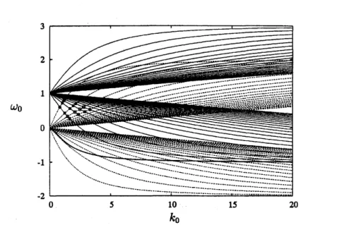
The

dispersion relation of Kelvin waves of$m=0$ (dashed lines) and $m=1$ (solid lines) is

displayed in figure 1. The isolated branchof$m=1,$startingfrom$\omega_{0}=0,$ isdrawnwitha

thick solidline. Infinitelymanybranchesemanatefrom $(k_{0}, \omega_{0})=$ _{$(0, 1)$} for$m=1$ among

which twenty branches, ten upgoing and ten downgoing, are drawn. Theses modes

are

named the radial modes since the eigenfunctions have nontrivial radial nodal structure.

A wave with $|\omega_{0}|>1$ rotatesfaster than the basic circulatory flow and iscalled

a

cograde

mode,which isdistinguished from

a

wave

with$|\omega_{0}|<1,$aretrogrademode (Sdman 1992).

In contrast,

an

isolated branch and the counterpart ofretrograde modes

are

missing for

the axisymmetric mode. Given the wavenumber $k_{0}$, the modes with $\omega_{0}$ and with $-?!0$

share

a

common

property ofcograde radial mode.

A positive axisymmetric mode $(\omega_{0}>0)$

crosses

every retrograde modeof$m=1$ once,

andmay cross, twice,

some

of higher cogradebranches of$m=1.$ Anegative axisymmetric

mode $(\omega_{0}<0)$ collides, ifitsbranch index is high enough, with some of retrograde radial

modes of$m=1,$ twice per each. The isolated mode of $m=1$

crosses

branches of$m=0$

at smallvalues of$k_{0}$

.

The growth rate (3.18) is calculated at many of intersection points. Collision of

eigen-values of the 0,1

waves

does not necessarily result in instability. Stability is lost only at

intersection points between positive branches of $m=0$ and retrograde radial modes of

$m=1,$ andotherwise this isnotthe

case.

This behaviour lies in starkcontrast with that

of the MSTW instability. In the latter case, every eigenvalue collision invites

paramet-ric

resonance

(Eloy

&

Le Dies 2001; Fukumoto 2003). The energetics holds the key to

distinguish non-resonant collisions from resonant ones,

as

will be described in

\S 4.3.

In Table 1,

we

list the evaluated values of the growth rate and the unstable

band-width for lowwavenumbers. The

first

three

rows

correspondto thefirstthree intersection

points ofthe first positive axisymmetric mode $(m=0)$ with retrograderadial modes of

$m$$=1,$ and

are

markedwith circles in figure 1. The next three

rows are

alongthesecond

mode of$m=0$ (thick dotes), and thelastthree along the third mode of$m=0$ (squares).

Sincethetorus center is

a

circleof radius $R$,

an

unstablemode isrealizableonlywhenthe

arclength $2\pi R$ coincides with

some

integral multiple of a half ofthe wavelength $2\pi/h$

.

150

$\omega_{0}$

Figure 1: Dispersion relation of the axisymmetric

wave

$m=0$ (dashed lines) and the

helical

wave

$m=1$ (solid lines)

on

the Rankine vortex. The isolated branch of$m=1$ is

shown with

a thidc

line.

$k_{0}$ $\omega_{0}$ $\sigma_{1\max}$ $\Delta k_{1}$

0.8134868347 0.5970895378 0.05434123370

0.1022075453

1.018687659

0.7162537484 0.007063858086

0.01725321243 1.136862167 0.7794574187 0.008676095366

0.02449637577

1.224505620

0.4217998862 0.03931853915

0.1093080415

1.650449151

0.5528357882 0.03769686682

0.1381880078

1.927505750

0.6329096309

0.004366456551 0.01889368333

1.464572874

0.3290672352 0.02466638188

0.08406115354

2.059092345

0.4537065585 0.01547299060

0.07032354299

2.472533079 0.5364030938

0.03273541819

0.1773468081

Table 1: Themaximumgrowth rate$\epsilon\sigma_{1\max}$ andthehalf-wi th$\epsilon\Delta k_{1}$ of unstable

151

$(\begin{array}{l}\prime\prime\nearrow\mathit{1}\acute{l}\prime.J’\prime\prime j’JJ\prime|.\mathrm{i}\iota_{}\mathrm{i}\mathrm{i}\mathrm{O}\mathrm{o}\end{array}.\backslash |’---\sim\backslash \backslash \backslash \backslash \backslash _{1}|’l..\backslash ‘ 3\mathrm{S}_{\iota_{\mathfrak{l}_{1}}}$

$\mathrm{i}\mathrm{i}\mathrm{i}_{\mathrm{I}}\mathrm{i}\mathrm{I}||...\backslash ..\cdot J^{\acute{\prime}}\backslash |)$ $.\iota_{\backslash }$

$\backslash \mathrm{j}_{\nwarrow_{\backslash }^{\backslash \mathit{1}^{j}}}^{\backslash }[searrow]^{\backslash }\mathrm{S}_{\backslash }\mathrm{i}\backslash \sim_{--\sim}^{\backslash }\backslash \sim_{\vee\cdot---}\cdot-’$ \prime\prime\prime

’/

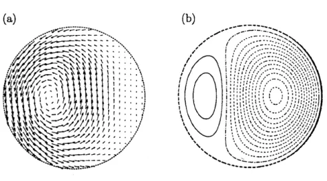
Figure 2: Contour ofdisturbance toroidal velocityfield$w_{0}$

on

the meridional plane$hs$ $=$

$\omega_{0}t$ for the first principal mode of the $(0, 1)$

resonance.

The dashed line depicts the

core

boundary$r=1.$

Large growth rate is maintained to short wavelengths at intersection points between

the $i$-th branch of $m=0$ andthe $i$-th branch of the retrograde radial modes of $m=1.$

Thissequence belongsto what wecall the principalmodes. The origin $(k_{0},\omega_{0})=(0,0)$is

the intersection point between the isolated branch of$m=1$ and all branches of $m=0.$

This is considered to be

a

neutrally stable point (Pukumoto

&

Hattori2004).

Amongtheintersection points examinedsofar,the maximum of growthrateisattained

at the first principal mode, namely at $(k_{0},\omega_{0})\approx$ (0.8134868347, 0.5970895378), though

the maximum value $\sigma_{1\mathrm{m}\mathrm{a}\mathrm{e}\mathrm{c}}\approx 0.05434123370$ is not very large. The correspon $\mathrm{i}\mathrm{g}$ flow

field is calculated, to $o(\epsilon^{0})$, from (3.8) with $v_{0}^{(1)}$ and $v_{0}^{(2}$) provided in Appendix A. The

solvability conditions bring in$\beta_{0}^{(2)}/\beta_{0}^{(1)}\approx$

0.7276318666

at this point.

The contour of toroidal velocity $w_{0}$ on the crosssectionalplane $k_{0}s=\omega_{0}t$ is drawn in

figure 2. Only the interior region $(r<1)$ is shown. A strong toroidal or axial current

is induced

over a

massive region with the location of peak velocity deviated backward

ffom the

core

center, and is accompanied by

a

minor counter current in the front part

ofthe core. The location of peak velocity winds helically around the torus center, and

executes

a

circulatory motion around the center. Figure $3(\mathrm{a})$ displays the disturbance

vorticity field $(\omega_{0r},\omega_{0\theta})$ of$O(\epsilon^{0})$ projected to the

same

crosssectional plane. The contour

oftoroidal vorticity$\omega_{0s}$ is shown in figure$3(\mathrm{b})$

.

The ring-lke vorticitystructure in figure

$3(\mathrm{a})$ corresponds to strong toroidal flow in figure 2. The toroidal vorticity is large at

points where the toroidal current is week.

We

reason

that,

as

withthe

cases

ofthe elliptical instability (Waleffe 1990) and of the

instability due to multi-polar strain (Eloy

&

Le Dizes 2001), the instability mechanism

is attributable to parallelization between the stretching direction of local shear and the

152

$1\{|$

(a) (b)

$.\neg.\sim\backslash -\approx..\simeq.*\sim$

Figure3: Disturbancevorticityfield in the meridional plane$k_{0}s=\omega_{0}t$of the firstprincipal

mode of the $(0, 1)$ resonance, (a) The meridional components $(\iota v_{0r},\omega_{0\theta})$

.

(b)

Contour

of

disturbance toroidal vorticityfield$\omega_{0s}$. The dashedline depicts the

core

boundary$r=1.$

function

of

angles between the disturbance vorticity vector and the eigenvectors of the

rate of strain for the first principal mode at $(k_{0},\omega_{0})\approx$ (0.8134868347, 0.5970895378).

Tendency ofalignment ofthe vorticityvector

was

recognized only with the unit toroidal

vector. It follows that vortex-line stretching in the toroidal direction plays the leading

role ofdriving instability.

The magnitudeofstrain increases with the distance $r$ from the

core

center and takes

its maximum at the

core

boundary $r=1.$ In the geometric-0ptics approximation, the

growth rate for the wave-packet disturbance of short wavelength attains its maximum

on the streamline circuiting the edge of the core (Hattori

&

Pukumoto 2003). In the

short-wave limit, onlythe disturbance vorticity

near

the

core

boundary isrelevant tothe

growthrate.

Thegrowthrate of theprincipalmodes diminishes

as

the branch labelbecomes larger.

Calculation of intersection points of the dispersion

curves

and of the growth rate

at

the

points is

extended

to large

wavenumbers

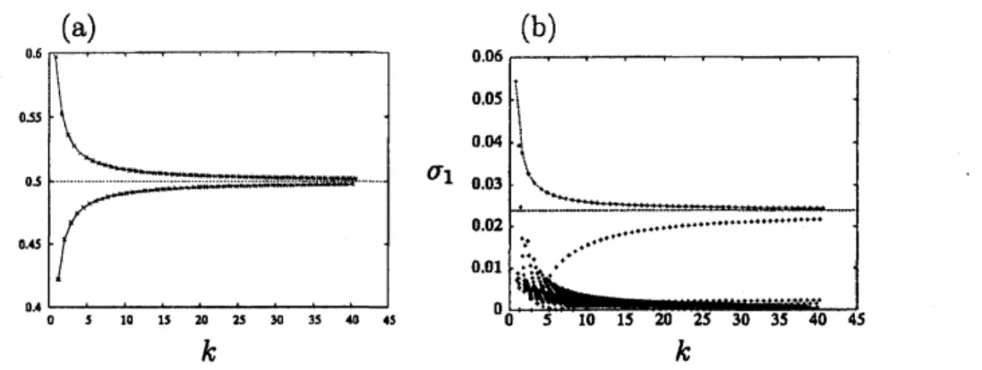
and isplottedin figure4. Thegrowthratestays

at relatively large values, approaching $\sigma_{1\max}\approx$ 0.02374715242, along the two sequences

of intersection points rapidly converging to $\omega_{0}=0.5$ (figure $4(\mathrm{a})$). One sequence is

intersection points between the $i$-th cograde mode of $m=0$ and the $i$-th retrograde

mode of$m=1$ forwhich the growth ratemonotonicallydecreases with$k_{0}$, andthe other

sequence is a collection of intersection points between the $(i+1)$-th cograde mode of

$m=0$ and the $i$-th retrograde mode of$m=1$ for which the growth rate is, except for

a

first few intersection points, an increasing function of $k_{0}$

.

Eloy

&

Le Dizes (2001) called

the latter the principal modes. We include both into the principal modes.

Inorderto graspoverall instabilitycharacteristics in the $(A_{0},\{v_{0})$ space, calculation of

153

$\omega_{0}$ _{$\mathrm{D}4_{\lambda^{\iota}}^{\iota_{\mathfrak{i}}}....\ovalbox{\tt\small REJECT} 9$} \

$\backslash .\cdot.\cdot\cdot..\ldots 2^{\cdot}0s$

.

$\mathrm{a}$

.

....

$k$ $k$

Figure 4: Large wavenumber behaviour of the $(0, 1)$ resonance, (a) The intersection

points $(k_{0},\iota v_{0})$ ofthe dispersion curves, (b) The maximum growth rate $\sigma_{1\max}$

.

over a

wide

range

of $k_{0}$ and _$m$

.

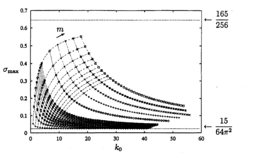
The growth rate is plotted in figure

5. The modes

of

$m=1,2$,$\cdots$,10 and 20, 30,$\cdots$,60

are

shown.

Given

_$m$, the growth

rate

of $(m, m+1)$

resonance

decreases with the branch label

or

the wavenumber $k_{0}$ and tends to $\sigma_{1\max}\approx$

0.02374715242 as

$k_{0}arrow\infty$

.

Onthe other hand, given the branch label, the growth rate

increases monotonicaUy with $m$ and approaches $\sigma_{1-}=$ 0.64453125

as

$marrow\infty$. The

ways ofapproachto thetwo different short-wave limits will be expounded in

\S 5.

4.2

Energetics

Krein’s theory of Hamiltonian spectra underlies the preceding numerical results. A

nec-essary conditionfor loss of stability at

a

double eigenvalue is either that the eigenfunction

consists of

waves

with opposite signed energy

or

that the eigenvalue is 0 (MacKay 1986;

Dellnitz, Melbourne

&

Marsden 1992; Knobloch, Mahalov

&

Marsden 1994).

By taking advantage of Cairns’ formula (Cairns 1979), Fukumoto (2003) reached

a

tidy expression for energy required to excite the Kelvin

wave

of azimuthal wavenumber

$m$

as

$E= \frac{2\pi\omega_{0}}{\omega_{0}-m}\{1+\frac{(k_{0}/\eta_{1})^{2}K_{|m|}(b)}{k_{0}K_{|m|-1}(k_{0})+|m|K_{|m|}(k_{0})}[$$\frac{2(\omega_{0}+\sqrt)}{\omega_{0}-m}$

$+( \frac{m(\omega_{0}+m)}{2}+k_{0}^{2}$

)

$\frac{K_{|m|}(k_{0})}{k_{0}K_{|m|-1}(k_{0})+|m|K_{|m|}(k_{0})}]\}(f_{0}^{(1)})^{2}$ _: (4.1)

where $f_{0}^{(1)}$ is the displacement amplitude ofthe disturbed

core

$r=1+f_{0}^{(1)}\exp[i(m\theta+$

$k_{0}z-\omega_{0}t)]$, and is linkedto the amplitude

56))

ofthe disturbance pressure through $f_{0}^{(1\rangle}= \frac{1}{4-(\omega_{0}-m)^{2}}\{-\eta_{m}J_{|m|-1}(\eta_{m})+\frac{|m|}{(v_{0}-m}(\omega_{0}-$

rn

$+ \frac{2m}{|m|}$

)

$J_{|m|}(\eta_{m})\}\beta_{0}^{(1)}$ (4.2)

By

a

computationof the above formula,

we

find thatthe energy of the axisymmetric

154

$A_{0}$

Figure 5: The growth rate of the principal modes between the $i$-th cogrademodes

of

_$m$

wave

and the$i$-thretrogrademodes of$m+1$

wave.

The

same

symbol isused

for

the

same

azimuthalwavenumber pair $(m, m+ 1)$

.

The lowestsequence $(+)$ _correspondsto$m=0.$

The highest sequence (0) correspondsto $m=60.$

energy

as

the$i$-th branch ofpositive mode. Theenergy of thebending

wave

$(m=1)$

was

illustrated in figure 8 of Fukumoto (2003). The energy of the isolated mode and cograde

radial modes of $m=1$ is positive

over

the entire range of $k_{0}$, and therefore

resonance

with the $m=0$ mode is ruled out. As is evident from (4.1), alteration of energy sign

occurs

at the point, $k_{0}^{*}$ say, where a dispersion

curve crosses

the $k_{0}$ axis. The energy of

retrograde radial modes of$m=1$ is negative intherange$0<k_{0}<k_{0}^{*}$, and is positive for

$t_{0}>I?.$ Eigenvaluecollisions of negative- and positive

energy

modes

occur

onlybetween

retrograde radial modes of $m=1$ and upgoing modes of $m=0$ in frequency

range

of

$0<\omega_{0}<1,$ being in

no contradiction

with the numerical example of

\S 4.1.

Krein’s criterion by

means

of the

energy

signature furnishes merely

a

necessary

con-dition for instability, yet it in effect

serves as a

sufficient condition for instability

as

well.

The

same

is true of the MSTW instability (Pukumoto 2003).

5

Short-wavelength

asymptotics

The expression (3.18) of growth rate suggests that

a

resonance

pair with $\omega_{0}$ closer to

$m+1/2$ is

more

influential. A universal feature manifests itself in the short wavelength

limit in which $\omega_{0}$ converges to $m+1/2$

.

Here

we

omit thederivation. Thedetail is found

in Fukumoto

&

Hattori (2004).

We have two wavelengths at

our

disposal, namely, theaxial and theazimuthal

155

azimuthal structure by fixing$m$, andthereafter

we

turnto the limit of$marrow\infty$.

5.1

Large

$k_{0}$

with

m

fixed

Let $l_{1}$ and$l_{2}$ be large integers indexing branches of the_$m$and the$m+1$wavesrespectively

as

$A_{0}$ with _$m$ fixed. Define

$\Delta l=l_{2}-l_{1\prime}$ $\Delta’l=2\Delta l-1$

.

(5.1)

Asymptotic expansions of $(k_{0},\omega_{0})$ for degenerate eigenvalues of the $m$,$m+1$

waves

are

manipulated from the dispersionrelation (A.7) and the counterpart of$m+$l. The

inter-section frequency is

$\omega_{0}=m+\frac{1}{2}+\frac{\sqrt{15}\pi\Delta’l}{128k_{0}}-\frac{1}{128A_{0}^{2}}\{m+\frac{1}{2}+\frac{\sqrt{15}\pi\Delta’l}{16}\}+O(A_{0}^{-3})$

.

(5.2)

The intersection wavenumber is obtained by solving iteratively

$k_{0}$ $=$ $\frac{1}{\sqrt{15}}\{\frac{\pi(l_{1}+l_{2}+m-1)}{2}+$$\arctan$ $( \frac{1}{\sqrt{15}})\mathrm{t}$ $- \frac{1}{30k_{0}}\{m^{2}+m+1+\frac{29\pi^{2}(\Delta’l)^{2}}{256}\}$

$+O(k_{0}^{-2})$

.

(5.3)

Substitutingfrom (5.2), (3.18) and (3.19) give,

$\sigma_{1\max}$ $=$ $\frac{15}{64\pi^{2}(\Delta’l)^{2}}+\frac{\sqrt{15}}{32k_{0}}\{\frac{m}{\pi\Delta’l}[\frac{21}{8}+\frac{1}{\pi^{2}(\Delta l)^{2}},]+\frac{1}{2}[$ $- \frac{9\sqrt{15}}{64}+\frac{21}{8\pi\Delta l}$

,

$+ \frac{\sqrt{15}}{16\pi^{2}(\Delta l)^{2}},+\frac{1}{\pi^{3}(\Delta l)^{3}},]\}+O(k_{0}^{-2})$ ,

$\Delta k_{1}$ $=$ $\frac{A_{0}}{2\pi^{2}(\Delta l)^{2}},+\frac{m}{\sqrt{15}\pi\Delta’l}[\frac{21}{8}+\frac{1}{\pi^{2}(\Delta l)^{2}},]+\frac{1}{2\sqrt{15}}[-\frac{\mathrm{g}\sqrt{15}}{64}+\frac{21}{8\pi\Delta l}$

,

$+ \frac{\sqrt{15}}{8\pi^{2}(\Delta l)^{2}},+\frac{1}{\pi^{3}(\Delta l)^{3}},]+O(k_{0}^{-1})$

.

(5.4)

Finite value $15/(64\pi^{2}(\Delta’l)^{2})$ of the growth rate is asymptoted in the limit of $A_{0}arrow$

$\infty$, among which the modes specified by $\Delta l=0$ and 1 have the largest growth rate

$15/(64\pi^{2})\approx$

0.02374715242.

This Umitingvalue is shared by allresonant pairs $(m, m+1)$

for finite values of$m$

.

These are the principal modes with slightlylarger growth

rate

for

$\Delta l=1.$ Correspondingly, the eigenfrequency $\omega_{0}$ of the principal modes with $\Delta l=0,1$

achieves

a

relatively rapid

convergence

to the limit$\omega_{0}=m+1/2$ from below and above

respectively as is

seen

from(5.2). Theunstable wavenumberband,toleading order,

broad-ens

linearly in $k_{0}$, and this broad-band nature guarantees the validity of the geometric

._{optics approachused by Hattori}

_&

_{Pukumoto (2003).}

Forthe principal modes, (5.4) become, for $\Delta l=1,$

$\sigma_{1\max}\approx$ $0.02374715242$$+0.02104135307/A_{0}$,

156

and, for $\Delta l=0,$

$\sigma 1\max\approx 0.02374715242-0.08399092777/A_{0}$,

$\Delta k_{1}$ $\approx$

0.05066059182

$k_{0}-$

0.1760143589

, (5.6)

They fit fairly well with the values shown in figure4.

Taking a careful look at figure $4(\mathrm{b})$ for the $(0,1)$ resonance, modes other than the

principal

ones

survive in the limit of $k_{0}arrow\infty$, which is confirmed ffom (5.4). This

situation is contrasted with the MSTW instability for which the $\Delta l=0$ mode holds a

specialstatus (Eloy

&

Le

Dizes

2001; Pukumoto 2003).

Notice that the coefficients of correction terms in the asymptotic expansions (5.2),

(5.3) and (5.4) grow with $m$, being indicative of nonuniformity in the expansions. At

largevalues of$m$

,

a new

regime shows up, inwhich vigorous modes reside.

5.2

Large

$k_{0}$

and m

with

_{$771\sim\eta_{2}\sim m$}

As $marrow\infty$, the intersection points $(k_{0},\omega_{0})$ between cograde radial modes of $m$ and

retrograde radial modes of$m+1$

are

arranged so

as

to satisfy $\eta_{1}\sim\eta_{2}\sim m$ (Eloy

&

Le

Dizes 2001). The asymptotic expansions for $(k_{0},\omega_{0})$ for those points

are

performed, to a

high order in $1/m^{1/3}$,

as

$k_{0}$ $=$ $\frac{m}{\sqrt{15}}-\frac{a_{1}+a_{2}}{2^{4}/\epsilon\sqrt{15}}m^{1/3}+\frac{1}{56}+\frac{1}{2\sqrt{15}}-\frac{49(a_{1}^{2}+a_{2}^{2})-290a_{1}a_{2}}{640\cdot 2^{1/3}\sqrt{15}m^{1/3}}$

$+ \frac{1}{87808\cdot 2^{1/3}}[\frac{2}{3\sqrt{15}}(-64429a_{1}+42477a_{2})-$ $725$($a_{1}+$a2)$] \frac{1}{m^{2/3}}+O(m^{-1})$,

(5.7)

$\mathrm{P}_{0}$

$=m+ \frac{1}{2}+\frac{15(a_{1}-a_{2})}{64\cdot 2^{1/3}m^{2/3}}+\frac{435}{1792m}+\frac{3(a_{1}^{2}-a_{2}^{2})}{64\cdot 2^{2/3}m^{4/3}}$

$+ \frac{5}{1404928\cdot 2^{1/3}}[2535\sqrt{15}$($-a_{1}+$ a2) $+169a_{1}+44073a_{2}] \frac{1}{m^{5/3}}+O(m^{-2})$

.

(5.8)

Inthese, $a_{1}(<0)$ and $\mathrm{Q}$ $(<0)$

are

the

zeros

ofthe AiryfunctionAiand play the role of the

branch labelsforthe$m$and the$m+1$

waves

respectively. The firstzero$a_{1}\approx$ -2.338107410

is tied with the first cograde radial mode of $m$ and $a_{2}\approx$ -2.338107410 with the first

retrograde radial mode of$m+$l.

A

rapid approach to $\omega_{0}=m+1/2$

as

$marrow$

oo

demands $\Delta a=$ _{a2 $-a_{1}=0.$} They sit

atthe crossing points between the $i$-th branches ofboth_$m$ and $m+$ $1$ radialwaves, and

thus

are

inherited fromtheprincipalmodes of$\Delta l=1.$ The growth rate

and

the

unstable

band

width for the

case

of$\Delta a=0$are, from (3.18)

and

(3.19),

$\sigma_{1\max}=$ $\frac{165}{256}(1-\frac{33499|a_{1}|}{25872\cross 2^{1/3_{\sqrt}2/3}})+O(m^{-1}$

)

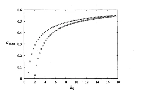
, (5.9) $\Delta k_{1}$ $=$ $8\mathrm{e}$$m(1- \frac{7627|a_{1}|}{25872\mathrm{x}2^{1}\mathit{1}^{3}m^{2/3}})+O(m^{0})$ (5.10)

157

0.6

$0.\mathrm{s}$

$\mathrm{x}^{\mathrm{x}^{\mathrm{x}^{\mathrm{x}_{\emptyset^{\mathrm{o}^{\mathrm{o}^{\mathrm{o}^{\mathrm{o}^{\mathrm{o}^{\mathrm{o}^{\circ^{\mathrm{o}^{\circ^{\mathrm{O}^{\circ \mathrm{O}}}}}}}}}}}}}^{\mathrm{x}^{\mathrm{x}^{\mathrm{x}^{\mathrm{x}^{\mathrm{x}^{\mathrm{x}^{\mathrm{x}\mathrm{o}\circ 0\circ \mathrm{o}\circ\circ \mathfrak{o}\mathfrak{o}\circ 0\circ\circ\circ 0\circ 6_{0}^{\mathrm{x}}\mathrm{s}\mathrm{a}_{\circ}^{\mathrm{X}}\mathrm{f}\mathrm{f}\mathrm{i}6\mathcal{B}\delta \mathrm{d}6\mathrm{f}\mathrm{f}\mathrm{i}b}}}}}}}}}}\mathrm{x}^{\mathrm{x}^{\mathrm{x}^{\mathrm{x}\mathrm{x}\mathrm{x}\mathrm{x}\mathrm{x}\mathrm{x}\mathrm{x}\mathrm{x}\mathrm{x}\mathrm{x}\mathrm{x}\mathrm{x}\mathrm{x}\mathrm{x}\mathrm{x}\mathrm{x}\mathrm{x}\cross \mathrm{X}}}}$

0.4 $\mathrm{x}\mathrm{x}^{\mathrm{x}^{\mathrm{x}_{\mathrm{O}}^{\mathrm{x}_{\mathrm{O}^{\mathrm{o}^{\mathrm{o}^{\mathrm{o}^{0}}}}}^{\mathrm{X}}}}}$ $\sigma-0.3$ $r\mathrm{x}\mathrm{x}$ $\circ\circ$ $\mathrm{x}$ $\circ$ $\mathrm{r}$ $\circ$ 0.2 $\mathrm{x}$ 0.1 $\mathrm{k}$ 0 0 2 4 6 8 10 12 14 16 18 $k_{0}$

Figure 6: Variation of the maximum growthrate$\sigma_{1\max}$ with$m$ for the

resonance

between

the first-first radial modes of the $m$, $m+1$ waves, $m=1,2$ ,$\cdots$, 60. The short-wave

asymptotics (5.11) and (5.7)

are

included with$\square$

.

The commonvalue $\sigma_{1-=}$ 165/256 is asymptoted. Among them, the longest

wave

pair

with $a_{1}=a_{2}\approx$ -2.338107410, the first principal mode, has the largest growth rate

$\sigma_{1\max}$ $\approx$ 0.64453125- $1.548698742/m^{2/3}$, (5.11)

$\Delta k_{1}$ $\approx$ 0.3550234734_$m$-0.1942235728$m^{1/3}$

.

(5.12)

This isthemostdominant mode

over

the all possible

resonance

pairs. Thewayof increase,

in $m$, of growth rate for the first principal mode is illustrated, with crosses, to $m=60$

in figure 6. It is worth noting that $\sigma_{1-}=165/256$ was derived through the geometric

opticsapproach byHattori

&

Fukumoto (2003). The present solution supplies

us

with its

structure globally in space.

In

case

$\Delta a=$ _a2 $-a_{1}\neq 0,$ convergence of the eigenvalue to $\omega_{0}=m+1/2$ is slower.

Modes with $\Delta a\neq 0$ vanish inthe limit of$marrow\infty$

.

A

Kelvin

waves

The expressions of the velocity field and the dispersionrelation ofKelvin

waves are

col-lectedinthis appendix. The leading-0rder disturbanceflowfieldof azimuthal wavenumber

$m$is obtained inthe form of normal mode as

$v_{0}=$

vSD

$(r)e^{\dot{*}m\theta}$., $\pi_{0}=\pi_{0}^{(1)}(r)e_{:}^{m\theta}\dot{.}$ $\phi_{0}=\phi_{0}^{(1)}(r)e^{|m\theta}$

.

158

By integratingthe linearized Eulerequations outsideand inside the

core

with radiusgiven

by (2.9), separately,

we

find that

$\phi_{0}^{(1)}=K_{m}(k_{0}r)\alpha_{0}^{(1)}$ for _{$r>1+\tilde{f_{0}}$} , (A.2)

and

$\pi_{0}^{(1)}=J_{m}(\eta_{1}r)\beta_{0}^{(1)}$ ,

$u_{0}^{(1)}= \frac{i}{\omega_{0}-m+2}\{-\frac{m}{r}J_{m}(\eta_{1}r)+\frac{\omega_{0}-m}{\omega_{0}-m-2}\eta_{1}J_{m+1}(\eta_{1}r)\}\beta_{0}^{(1)}$,

$v_{0}^{(1)}= \frac{1}{\omega_{0}-m+2}\{\frac{m}{r}J_{m}(\eta_{1}r)+\frac{2}{\omega_{0}-m-2}\eta_{1}J_{m+1}(\eta_{1}r)\}\beta_{0:}^{(1)}$

$UJ_{0}(’$ $= \frac{k_{0}}{\omega_{0}-m}J_{m}(\eta_{1}r)\beta_{0}^{(1)}$ for $r<1+\tilde{f}_{0}$, (A.3)

where the radialwavenumber $\eta_{1}$ is given by

$\eta_{1}^{2}=[4/(\omega_{0}-m)^{2}-1]k_{0}^{2}$ , (A.4)

and $J_{m}$ and $K_{m}$

are

respectively the Bessel function ofthe ffist kind and the modified

Bessel function of the second kind, $m$ being their order, and $\alpha_{0}^{(1)}$ and $79^{1)}$ are arbitrary

constants.

The non-singular conditions $\omega_{0}f$_$m$ and $\omega_{0}\neq m\mathrm{i}$ $2$

are

to be kept in view.

The

radial

wavenumber of the $m+1$

wave

is

$\eta_{2}^{2}=[4/(\omega_{0}-m-1)^{2}-1]A_{0}^{2}$

.

(A.5)

The boundaryconditions supplythe relation between $\alpha_{0}^{(1)}$ and$\beta_{0}^{(1)}$

as

$\alpha_{0}^{(1)}=-\frac{iJ_{m}(\eta_{1})}{(\omega_{0}-m)K_{m}(k_{0})}79^{1)}$

: (A.6)

and the dispersion relation

$J_{m+1}( \eta_{1})=\{\frac{2m}{\omega_{0}-m+2}-\frac{k_{0}K_{m+1}(A_{0})}{K_{m}(k_{0})}\}\frac{\eta_{1}}{k_{0}^{2}}J_{m}(\eta_{1})$

.

(A.7)

B

Closed-form solution for disturbance field and the

solvability

conditions

Thisappendix isconcernedwiththe closed-formsolutionof the$O(\epsilon)$disturbancefield, the

boundary conditions, and the solvability conditions for

a

possible parametric

resonance

between Kelvin

waves

with azimuthal wavenumbers $m$and$m1$ $1$

.

Thesuperscript 1 refers

159

By inspection and with the help ofcomputer algebra, a generalsolution of (3.13) for

the $m$ wave, finite at $r=0,$ is manipulated as

$\pi \mathrm{P})$ $=J_{m}( \eta_{1}r)\beta_{1}^{(1)}+\{\frac{4k_{0}^{2}\omega_{1}}{(\omega_{0}-m)^{3}}-\frac{\eta_{1}^{2}A_{1}}{k_{0}}$

}

$\frac{r}{\eta_{1}}J_{m+1}(\eta_{1}r)\beta_{0}^{(1)}$

$+ \frac{i}{16}\{[5(r^{2}-1)+\frac{(\omega_{0}-m-1)^{2}(\omega_{0}-m)^{2}(\omega_{0}-m+2)}{2k_{0}^{2}(2\omega_{0}-2m-1)^{2}(\omega_{0}-m+1)}A_{1}]\eta_{2}J_{m}(\eta_{2}r)$

$+ \frac{A_{2}}{2\omega_{0}-2m-1}rJ_{m+1}(\eta_{2}r)\}\mathrm{j}3_{0}^{(2)}$, (B.1)

where $3(^{1)}$ is a constant and

$A_{1}$ $=9\omega_{0}^{4}-18(2m+1)\omega_{0}^{3}+(54m^{2}+54m+1)\omega_{0}^{2}-2(2m+1)(3m-2)(3m+5)\omega_{0}$

$+977$$4+18m^{3}-23m^{2}-32m-$ $8$,

$A_{2}$ $=9\omega_{0}^{4}-$ $9(4m+1)\omega_{0}^{3}+(54m^{2}+27m-26)\omega_{0}^{2}-(36m^{3}+27m^{2}-56m-20)\omega_{0}$ $+9\mathrm{v}\mathrm{n}^{4}$ $+9m^{3}-30m^{2}-$_$22$

$m-$ $2$

.

(B.2)

Returning to the Euler equations (3.1) and (3.2), the disturbance radial velocity$u_{1}^{(m)}$ is

found to be

$u_{1}^{(1)}=i \{-\frac{mJ_{m}(\eta_{1}r)}{(\omega_{0}-m+2)r}+\frac{1}{2}(\frac{1}{\omega_{0}-m+2}+\frac{1}{\omega_{0}-m-2})\eta_{1}J_{m+1}(\eta_{1}r)\}\beta_{1}^{(1)}$

$+ \frac{i\omega_{1}}{(\omega_{0}-m+2)^{2}}\{[\frac{m}{r}+\frac{4\eta_{1}^{2}r}{(\omega_{0}-m-2)^{2}}]J_{m}(\eta_{1}r)$

$- \frac{1}{(\omega_{0}-m-2)^{2}}[\omega_{0}^{2}-2m\omega_{0}+(m+2)^{2}+\frac{8m}{\omega_{0}-m}]\eta_{1}J_{m+1}(\eta_{1}r)\}\beta_{0}^{(1)}$

$-iA_{1} \{\frac{k_{0}}{\omega_{0}-m}rJ_{m}\mathrm{C}’/\mathrm{i}^{\mathrm{V})}$$+ \frac{m}{A_{0}(\omega_{0}-m-2)}71J_{m+1}(\eta_{1}r)\}\beta_{0}^{(1)}$

$+ \frac{1}{16}\{\frac{1}{\omega_{0}-m+1}[$$m( \frac{(\omega_{0}-m)^{2}(\iota v_{0}-m-1)^{2}}{2k_{0}^{2}(2\omega_{0}-2m-1)^{2}}A_{1}-5)\frac{1}{r}$

$+ \frac{A_{3}}{(\omega_{0}-m-3)(2\omega_{0}-2m-1)}r]\eta_{2}J_{m}(\eta_{2}r)$ $+[ \frac{A_{4}}{2(\omega_{0}-m-3)(2_{\mathfrak{l}}v_{0}-2m-1)^{2}}+\frac{5k_{0}^{2}}{\omega_{0}-m-1}(r^{2}-1)]J_{m+1}(\eta_{2}r)\}\beta_{0}^{(2)}$ , (B.3) where

A3

$=$ $9\omega_{0}^{5}-9(5m+3)\omega_{0}^{4}+$ ($90m^{2}+$108m$+1$)$\omega_{0}^{3}-(90m^{3}+162m^{2}-11m-11)\omega_{0}^{2}$ $+(45771^{4}+108m^{3}-25m^{2}-63m+14)\omega_{0}-9m^{5}-27m^{4}+13m^{3}+52m^{2}+3m-8$ ,

ieo

$-8)\omega_{0}^{5}+(630m^{4}+1890m^{3}+1290m^{2}-98m-87)\omega_{0}^{4}$ $-2(252m^{5}+945m^{4}+880m^{3}-116m^{2}-262m-27)\omega_{0}^{3}$ +2$(126m^{6}+567m^{5}+675m^{4}-134m^{3}-533m^{2}-154m+18)\omega_{0}^{2}$ -2$(36m^{7}+189m^{6}+276m^{5}-76m^{4}-454m^{3}-235m^{2}+32m+28)\omega_{0}$ $+9m^{8}+54m^{7}+94m^{6}-34m^{5}-$$279m^{4}-$_{$216m^{3}+24m^{2}+68m+16$}

.

_(B.4)

Substituting from (3.11), (B.$\mathrm{I}$), (B.3) and theexpressions in Appendix

A

and

evalu-ating them at $r=1,$ the boundaryconditions (3.16) for the $m$

wave are

converted into

linear algebraic equationsfor $\alpha_{1}^{(1)}$ and$\beta \mathrm{g}1$):

$[mK_{m}-k_{0}K_{m+1}-i(\omega_{0}-m)K_{m}$ $\frac{1}{\omega 0-m+2}[mJ_{m}(\eta_{1})-\frac{w\mathrm{o}-m}{\mathrm{t}d\mathrm{p}-m-2,1)},$$/\mathrm{i}^{\mathrm{j}_{m+1}(\eta_{1})]}J_{m}(\eta][_{\beta_{1}^{(1)}}\alpha_{1}^{(1)}]=\{\begin{array}{l}F^{(1)}G^{(1)}\end{array}\}$ ,

(B.5) wherewehave madeuseof theshorthand notation$K_{m}=K_{m}(k_{0})$ and$K_{m+1}=K_{m+1}(k_{0})$

.

Thedispersionrelation (A.7) helps to simplify$F^{(1)}$ and$G^{(1)}$ byeUminating $J_{m+1}(\eta_{1})$from

these equations.

As

isusuallythe case, thematrix in (B.5) is singular, and hence the vector $(F^{(1)}, G^{(1)})$

must be constrained to its image space in order for (B.5) to be solvable for $(\alpha_{1}^{(1)}, 5\mathrm{P}^{)})$

.

This solvability condition reads

$i( \omega_{0}-m)F^{(1)}+(m-\frac{A_{0}K_{m+1}}{K_{m}})G^{(1)}=0$

.

(B.5)

The

same

procedure is repeated for the$m+$$1$

wave.

These conditions

are

rewritten into homogeneous linear algebraic equations for $65^{1)}$

and $\beta_{0}^{(2)}$

as

$\{\frac{\omega_{1}f^{(1)}}{(\omega_{0}-m+2)(\omega_{0}-m-2)}+\frac{2k_{1}}{k_{0}}(\omega_{0}-m)g^{(1)}\}\beta_{0}^{(1)}$ $+ \frac{i(\iota v_{0}-m)^{4}J_{m+1}(\eta_{2})}{32k_{0}^{2}(2\omega_{0}-2m-1)^{2}(\omega_{0}-m-1)J_{m}(\eta_{1})}h\beta_{0}^{(2)}=0$ , (B.7) $- \frac{\overline{\iota}(\omega_{0}-m-1)^{4}J_{m}(\eta_{1})}{32k_{0}^{2}(2\omega_{0}-2m-1)^{2}(\omega_{0}-m)J_{m+1}(\eta_{2})}h\beta_{0}^{(}$’ $+\{$$\frac{\omega_{1}f^{(2)}}{(\omega_{0}-m+1)(\omega_{0}-m-3)}+\frac{2k_{1}}{k_{0}}(\omega_{0}-m-1)g^{(2)}\}\beta_{0}^{(2)}=0$

.

(B.8) Inthese,

$f^{(1)}$ $=$ $m[\omega_{0}^{3}- (3\mathrm{v}\mathrm{r}\mathrm{z} + 4)\omega_{0}^{2}+ 3\mathrm{v}\mathrm{r}\omega_{0}-270(m^{2}- 4\mathrm{r}\mathrm{n}-8)]$ $+2k_{0}^{2}(\omega_{0}-m)^{2}$

$+4[(771+1) \omega_{0}^{2}-2m^{2}\omega_{0}+m(m^{2}-m-4)]\frac{k_{0}K_{m+1}}{K_{m}}$

181

$f^{(2)}$ _$=$ $(m+1)[\omega_{0}^{3}-(3m-1)\omega_{0}^{2}+3(m+1)^{2}\omega_{0}-m^{3}-7m^{2}-3m+3]$ $+2A_{0}^{2}( \omega_{0}-m-1)^{2}-4[m\omega_{0}^{2}-2(m+1)^{2}\omega_{0}+(m+1)(m^{2}+3m-2)]\frac{A_{0}K_{m}}{K_{m+1}}$ $-2( \omega_{0}-m+1)(\omega_{0}-m-3)\frac{k_{0}^{2}K_{m}^{2}}{K_{m+1}^{2}}$, (B.13) $g^{(1)}$ _{$=$ $-(m- \frac{k_{0}K_{m+1}}{K_{m}})[m(\omega_{0}-m-1)+\frac{k_{0}K_{m+1}}{K_{m}}]$} , (B.13) $g^{(2)}$ _$=$ $(m+1+ \frac{k_{0}K_{m}}{K_{m+1}})[(m+1)(\omega_{0}-m)+\frac{k_{0}K_{m}}{K_{m+1}}]$ _: (B.12) $h=( \omega_{0}-m)(\omega_{0}-m-1)\{(m+1)(\omega_{0}-m+2)\frac{k_{0}K_{m+1}}{K_{m}}+$ $\mathrm{t}\mathrm{n}(\omega_{0}-m-3)\frac{k_{0}K_{m}}{K_{m+1}}$ -2$m(m+1) \}A_{1}+2k_{0}^{2}A_{5}+(2\omega_{0}-2m-1)k_{0}^{3}\{[A_{1}-6(3\omega_{0}^{2}-3\omega_{0}-3m^{2}+1)]\frac{K_{m+1}}{K_{m}}$ $-[A_{1}-6(3\omega_{0}^{2}+3\omega_{0}-3m^{2}-6m- 2)]$$\frac{K_{m}}{K_{m+1}}\}$, (B.13) where $A_{5}$ $=$ $9\omega_{0}^{6}-36(2m+1)\omega_{0}^{5}+(225m^{2}+225m+46)\omega_{0}^{4}-9(2m+1)(20m^{2}+20m-3)\omega_{0}^{S}$ $+(315m^{4}+630m^{3}+126m^{2}-189m-38)\omega_{0}^{2}$ $-\mathrm{m}(\mathrm{m}+1)(2\mathrm{m}+1)(72m^{2}+72m-115)\omega_{0}$ $+27m^{6}+81m^{5}+12m^{4}-111m^{3}-71m^{2}-2m+4$

.

(B.14)

References

[1] BAYLY, B. J.

1986

Three-dimensional instability ofelliptical flow. Phys. Rev. Lett.

57, 2160-2163.

[2] CAIRNS, R. A. 1979 The role of negativeenergy

waves

in

some

instabilities of parallel

flows. J. Fluid Mech. 92, 1-14.

[3] DELLNITZ, M., MELBOURNE, I.

&

MARSDEN, J. E. 1992 Generic bifurcation of

Hamiltonian vector fields with symmetry. Nonlinearity 5, 979-996.

[4] Eloy,

C.

&

LE

DIZ\‘ES,

S. 2001 StabilityoftheRankine vortex inamultipolar strain

field. Phys. Fluids 13, 660-676.

[5] Fukumoto, Y.

2002

Higher-0rder asymptotic theory for the velocity

field

induced

by

an

inviscid vortexring. Fluid Dyn. ${\rm Res}$

.

30,

67-95.

[6] Fukumoto, Y. 2003 The three dimensional instability of

a

strained vortex tube

162

[7] Fukumoto, Y.

&

HATTORI, Y. 2002 Linear stability of

a

vortex ring revisited.

In Proc.

_of

IUTAM

Symposium

on

Tabes, Sheets and Singularities in Fluid Dynamics

(eds. H. K. Moffatt and K. Bajer), pp.

37-48.

Kluwer.

[8] Fukumoto, Y.

&

HATTORJ, Y. 2004Curvatureinstability of

a

vortexring. preprint.

[9] Fukumoto, Y.

&

MOFFATT, H. K. 2000 Motion and expansion of a viscous vortex

ring. Part 1. A higher-0rder asymptotic formula for the velocity. J. Fluid Mech. 417,

1-45.

[10] HATTORI, Y.

&

Fukumoto, Y. 2003 Short-wavelength stability analysis of thin

vortex rings. Phys. Fluids. 15, 3151-3163.

[11] KNOBLOCH, E., MAHALOV, A.

&

MARSDEN, J. E. 1994 Normalforms for

three-dimensional parametric instabilities in idealhydrodynamics. Physica D73, 49-81.

[12] MACKAY, R.

S. 1986

Stability

of

equilibria

of

Hamiltonian systems.

In

Nonlinear

Phenomena and Chaos (ed. S. Sarkar),

pp. 254-270.

Adam Hilger, Bristol.

[13] Moore, D. W.

&

SAFFMAN, P.

G.

1975 The instability of a straight vortex

filament in

a

strain field. Proc. R. Soc. Lond. A 346, 413-425.

[14] SAFFMAN, P.

G.

1992 VortexDynamics, Chap. 12. Cambridge University Press.

[15] Tsai, C.-Y.

&

WIDNALL, S. E. 1976 The stability of short

waves

on

a straight

vortexfilament in a weak externaly imposed strainfield. J. Fluid Mech. 73, 721-733.

[16] WALEFFE, F. 1990 On the three-dimensional instability of strained vortices. Phys.

Fluids A 2,

76-80.

[17] WIDNALL, S. E., BLISS, $\mathrm{D}^{\cdot}$

.

B.

&

Tsai,

C.-Y. 1974

The instabilityofshort

waves

on a

vortexring. J. Fluid Mech. 66, $35\triangleleft 7$

.

[18] WIDNALL, S. E.

&

Tsai,

C.-Y.

1977

The instability of the thin vortex ring of