Asymptotic Behavior of Solutions for an Interface Equation : Interface Dynamics and Center-of-Mass Motions (Evolution Equations and Asymptotic Analysis of Solutions)

(1)

Asymptotic Behavior of Solutions for

an

Interface Equation

– Interface Dynamics and Center-of-Mass

Motions

–

広島大学大学院理学研究科岡田浩嗣 (Koji Okada)

Graduate School of Science, Hiroshima University

1 INTRODUCTION

In 1992, Rubinstein

&

Sternberg proposed in [9] the following scalar bistable

reaction-diffusion equation with a nonlocal term:

(NL) $\{$

$u_{t}^{\epsilon}= \epsilon^{2}\triangle u^{\epsilon}+f(u^{\epsilon})-\frac{1}{|\Omega|}\int_{\Omega}f(u^{\epsilon})dx$,

$\partial u^{\epsilon}/\partial \mathrm{n}=0$,

$t>0$

,

$x\in\Omega$,

t>0ラ $x\in\partial\Omega$

.

Here,

0

is a smooth boundeddomainin$\mathbb{R}^{N}(N\geq 2)$ with volume $|\Omega|$ and the outward

unit normal $\mathrm{n}$ on the boundary

$\partial\Omega$, _$\epsilon>0$ is a small parameter, and _$f$ is a function

derived from a double-wellpotential, a typical example being $f(u)=u-u^{3}$.

It is known that the dynamics of solutions for (NL) with $\epsilon<<1$ consists of several

stages, and is roughly summarized as follows.

(51) Generation of transition layers [9]:

The solution with an appropriate initial condition generates sharp transition

layer near an interface. Such a solution is referred to as a layer solution.

(52) Motion ofinterfaces (i) [9]:

Thelayer solution begins to evolve so that the corresponding interface is driven

according to a certain motion law, called an interface equation. The interface

equation is given by (2.15) in [9].

(53) Motion of interfaces (ii) [9]:

The layer solution then comes to evolve so that the corresponding interface is

governed by another interface equation, which is well-know$\mathrm{n}$ as the volume

preserving mean curvature flow (cf. [5, 6, 7]). The interface is driven in such

a way that the volume enclosed by the interface is preserved and the area of

the interface decreases. After a coarsening process, the interface evolves into a singlesphere. The layer solution withsphericalshape is referredto as the bubble

solution.

(54) Motion of bubbles (i) [1, 3, 11, 12]:

Thebubble solution drifts withexponentiallyslow speed without changing shape

toward the closest point on

an

from the center of the corresponding sphere.

(55) Motion ofbubbles (ii) $[2, 12]$:

Oncethe bubblesolution attaches to

an,

it intersects perpendicularlyto

an

and

(2)

The dynamics in $(\mathrm{S}1)-(\mathrm{S}3)$ was formally discussed in [9] by employing asymptotic

analysis. For (S4), the existence of such bubble motions was established by Alikakos

et al. [1]. Ward gave in [11] an explicit asymptotic ordinary differential equation for

the distance between the center ofthe bubble and the closest point on af (see also [12]$)$

.

Alikakos et al. derived in [3] such an equation for the Cahn-Hilliard equation

and compared the bubble motions for the

Cahn-Hilliard

equation with those for the

nonlocal equation (NL). The dynamics in (S5) was studied by Alikakos et al. [2].

Our concernin this paper is the dynamicsoccurringinthe intermediatestage (S2),

i.e.,

_after

the formation of layers and

_before

the volume-preserving

mean curvature

flow iseffective. The corresponding interfaceequation was earlier given byRubinstein

&

Sternberg as (2.15) in [9]. The form, however, was implicit and unsuitable for

the circumstantial examinationfrom interfacial approach. We will present below an

explicitformulationof theinterfaceequation, and discuss the dynamicsand asymptotic

behavior of solutions for the interface equation. Throughout the remaining of this

paper, an “interface” means a smooth, closed, $(N-1)$-dimensional hypersurface $\Gamma$

embeddedin$\Omega\subseteq \mathbb{R}^{N}$staying uniformly away from

an.

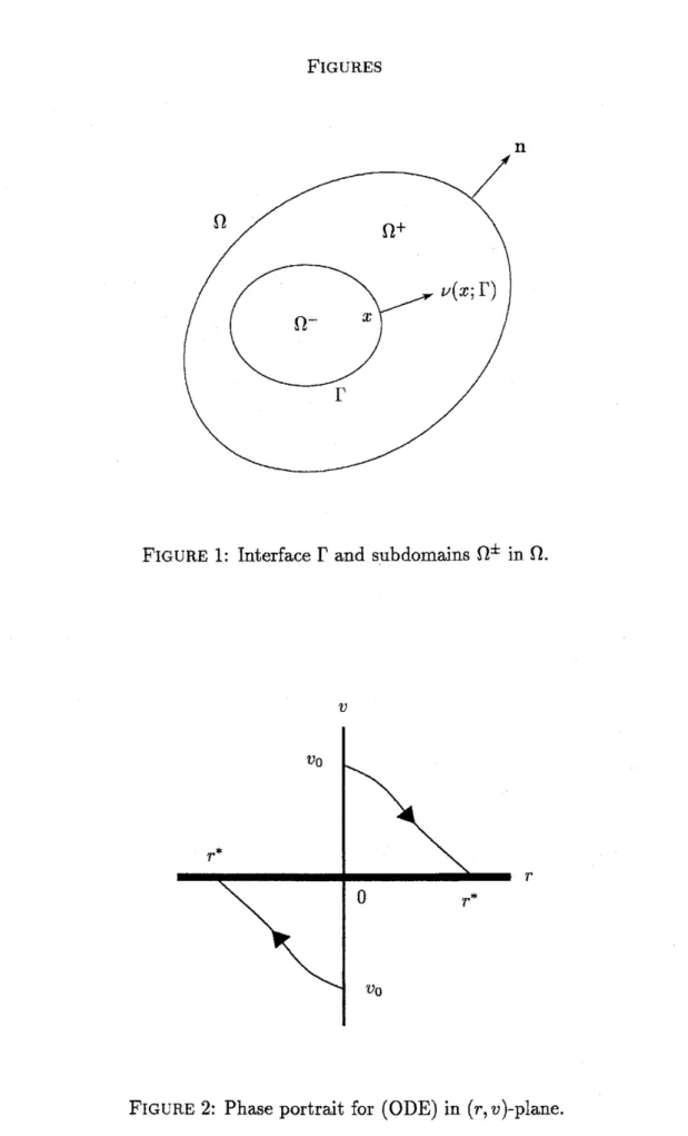
We denote by$\Omega^{\pm}$ subdomains

in $\Omega$ separated by an interface $\Gamma$ such as

$\Omega=\Omega^{-}\cup\Gamma\cup\Omega^{+}$,

an-

$=\Gamma$, $\partial\Omega^{+}=\partial\Omega\cup\Gamma$,

and by $\nu(x;\Gamma)$ the unit normal vector on $\Gamma$ at _$x\in\Gamma$ pointing toward the interior of

the subdomain $\Omega^{+}$

(cf. FIGURE 1).

Let $\{\Gamma(t)\}_{t\geq 0}$ be a family of interfaces parameterized by time $t\geq 0$

,

with each

interface $\Gamma(t)$ satisfying the conditions above. The interface equation associated with

the intermediatestage (S2) is explicitly given as follows (cf. [8]):

(IE-a) $\mathrm{v}(x;\Gamma(t))=c(v(t))$, $t>0_{;}x\in\Gamma(t)$,

(IE-b) $\dot{v}(t)=\frac{h^{+}(v(t))-h^{-}(v(t))}{h_{\overline{v}}(v(t))|\Omega^{-}(t)|+h_{v}^{+}(v(t))|\Omega^{+}(t)|}c(v(t))|\Gamma(t)|$

,

t $>0$,

(IE-c) $\Gamma(0)=\Gamma_{0}$

,

$v(0)=v_{0}$.

Here, $\mathrm{v}(x;\Gamma(t))$ denotes the normal velocity of $\Gamma(t)$ at $x\in\Gamma(t)$ in $\nu$-direction, the

symbols $|\Gamma(t)|$ and $|\Omega^{\pm}(t)|$ stand forthesurfacearea of$\Gamma(t)$ and thevolumesof$\Omega^{\pm}(t)$

,

respectively, $c(v)$ and $h^{\pm}(v)$ are some functions defined in a neighborhood of $v=0$

satisfying

(1.1) $c(0)=0$, $c’(0)>0$; $h^{-}(v)<0<h^{+}(v)$, $h_{v}^{\pm}(v)<0$

.

The interface equaiton (IE) is derived in [8] as a singular limit of the following

problem

(RD) $\{$

$\epsilon u_{t}^{\epsilon}=e^{2}\Delta u^{\epsilon}+f(u^{\mathrm{e}})-v^{e}$

,

$t>0$

,

$x\in\Omega$,

$v^{\epsilon}=$ $\frac{1}{|\Omega|}\int_{\Omega}f(u^{\epsilon})dx$, $t\geq 0$

,

(3)

as $\epsilonarrow 0$, where the problem (RD) is obtained by rescaling the time $t$ in (NL) as

$t\vdasharrow\epsilon^{-1}t$and introducing an auxiliary variable for the nonlocal term. Inthissituation,

thefunctions$\mathrm{I}^{\pm}(v)$, $c(v)$in (IE) satisfying(1.1) aredetermined by thethenonlinearity

$f(u)-v$ in (RD). We should also mentionthat $\Gamma(t)$ and $v(t)$ in (IE) correspond to

limits ofthe level-set interface $\Gamma^{\epsilon}(t):=\{x\in\Omega|u^{\epsilon}(t, x)=0\}$ and the nonlocal term

$v^{\epsilon}(t)$ in (RD) as $\epsilonarrow 0$, respectively, and that $u^{\epsilon}$ with $\epsilon\ll 1$ has

a

sharp layerstructure

near $\Gamma(t)$ such as

$u^{\epsilon}(t, x)\approx h^{\pm}(v(t))$, $t>0$, $x\in\Omega^{\pm}(t)$.

By virtue of the precise formulations as (RD) and (IE), the unique existence of

time local and global solutions to (IE) and the convergence of solutions for (RD) to

those for (IE) have been successfully established in [8]. In paticular, the convergence

result

guarantees

that the dynamics of solutions for (IE) does approximate that for

(NL) in the intermediate stage (S2). In this sense, it is of crucial importance to

ex amine thedynamics and asymptoticbehavior of solutions to (IE) for understanding

the dynamics occurring in (S2).

2 INTERFACE DYNAMICS

By the conditions in (1.1), it is easily verified that the dynamics of $(\Gamma(t), v(t))$ is

as follows:

(i) $v$ $>0$ $\Rightarrow$ $\mathrm{v}>0,\dot{v}<0$;

$\Gamma(t)$ evolvesin sucha waythat$\Omega^{-}(t)$ grows (or$\Omega^{+}(t)$ shrinks) and$v(t)$ decreases.

(ii) $v<0$ $\Rightarrow$ $\mathrm{v}<0,\dot{v}>0$;

$\Gamma(t)$ evolvesin sucha waythat $\Omega^{-}(t)$ shrinks (or$\Omega^{+}(t)$ grows) and $v(t)$ increases.

(iii) $v=0$ $\Rightarrow$ $\mathrm{v}=0,\dot{v}=0$;

$\Gamma(t)$ and $v(t)$ do not evolve.

The description above is the same as that in [9]. To examinethe asymptoticbehavior

ofsolutions for (IE), we will recast (IE) as an equivalent problem.

2.1

Preliminaries.

Beforemoving on, we prepareinthis subsectionnotations and

tools neededlater.

For$t\geq 0$, we express$\Gamma(t)$ as a smooth embeddingfrom a fixed$(N-1)$-dimensional

reference manifold $\mathcal{M}$ to $\mathbb{R}^{N}$:

(2.1) $\gamma(t, \cdot)$ : $Marrow\Gamma(t)$, $M$ $\ni y\vdash\Rightarrow x=\gamma(t, y)\in\Gamma(t)$

.

Let $\nu(t, y)\in \mathbb{R}^{N}$ be theunit normal vector$\nu(x;\Gamma(t))$ on $\Gamma(t)=\gamma(t, M)$ at $x=\gamma(t, y)$.

We

normalize

the

parametrization

(2.1) so that $\gamma_{t}$ is always parallel to

$\nu$

.

This yields

that $\gamma_{t}=\mathrm{v}\mathrm{v}$. We simply denote by

$\varphi(y)$ and $n(y)$ instead of $\gamma(0, y)$ and $\nu(0, y)$,

respectively. For sufficient small $|r|$

,

we define the embedding$F(r$,$\cdot$$)$ : $M$ $arrow\Omega$ as

(4)

Then the hypersurface defined by

(2.2) $\Gamma_{r}:=F(r, M)=\{x\in\Omega|x=\varphi(y)+rn(y), y\in.M\}$

is smoothforsmall $|r|$. Let $dS_{y}^{f}$ be thevolumeelement on $M$ inducedfrom thesurface

element on $\Gamma_{f}=F$($r$,A4) at $x=F(r, y)$ by the embedding$F(r$,$\cdot$$)$

.

Note that $dS_{y}^{r}$ has

the following expressions:

$dS_{y}^{r}$ $=$ $\prod_{j=1}^{N-1}(1+r\kappa_{j}(y))dS_{y}^{0}$

$=$: $\sum_{j=0}^{N-1}H_{j}(y)r^{j}dS_{y}^{0}$.

Here, $\kappa_{j}(y)(j=1, \cdots : N-1)$ stand for the principal cuvatures of $\Gamma_{0}=\varphi(M)$ at

$x=\varphi(y)$ and $H_{j}(y)(j=0, \cdots : N-1)$ are the fundamental symmetric functions of

$\kappa_{1}(y)$,$\cdot$.. ,$\kappa_{N-1}(y)$:

$H_{0}(y)$ $\equiv$ 1, $H_{1}(y)$ $=$ $\kappa_{1}(y)+\cdots+\kappa_{N-1}(y)$,

.

$\cdot$

.

$H_{N-1}(y)$ $=$ $\kappa_{1}(y)\cdots\kappa_{N-1}(y)$

.

The surface area $|\Gamma,|$ is denotedby $g(r)$

.

Then $g(r)$ is explicitly givenby

(2.3) $g(r)= \sum_{i=0}^{N-1}(\oint_{\mathcal{M}}H_{i}(y)dS_{y}^{0})r^{j}$.

2.2 Asymptoticbehavior of solutions. Let

us

now

recast

(IE) as an equivalent

problem.

For a given initial interface $\Gamma_{0}$, we express the interface $\Gamma(t)$ as the graph of a

function $r(t,$y) over $\Gamma_{0}$:

(2.4) $\Gamma(t)=$

{x

$\in\Omega|x=\gamma(t, y)=\varphi(y)+r(t, y)n(y),$y $\in M\}$

.

A simple computation implies that $\nu(t,$y) is independent oft $>0$:

(2.5) $\nu(t, y)\equiv n(y)$

.

From (2.4), (2.5) and

v

$=\gamma_{\mathrm{t}}\cdot$$\nu$, the equation in (IE-a) now turns out to be expressed

as $r_{t}(t, y)=c(v(t))$

.

The initial condition for $\mathrm{T}(\mathrm{t})$ in (IE-c) is recast in terms of r as

$r(0, y)=0$. Then the equation for $a(t,y):=\nabla_{y}r(t,$y) becomes $a_{t}(t, y)=0$

,

$a(0, y)=0$,

from which it follows $a(t, y)\equiv 0$, i.e., $r(t,$y) is independent ofy $\in \mathcal{M}$:

(5)

Therefore, the equation in (IE-a) with the initial condition in (IE-c) is recast as

$\dot{r}(t)=c(v(t))$

,

$r(0)=0$.

By (2.4) and (2.6), the interface $\Gamma(t)$ is expressed as

$\Gamma(t)=\{x\in\Omega|x=\varphi(y)+r(t)n(y), y\in\Lambda \mathit{4}\}$$=\Gamma_{f(t)}$,

while thesurface

area

$|\Gamma_{r}|$ is given by (2.3), Thus wehave $|\Gamma(t)|=g(r(t))$

.

On the other hand, thefollowing identities are valid:

$\frac{d}{dt}|\Omega^{-}(t)|=-\frac{d}{dt}|\Omega^{+}(t)|=\int_{\Gamma(t)}\mathrm{v}(x;\Gamma(t))dS_{x}^{\Gamma(t)}$

,

where $dS_{x}^{\Gamma(t)}$ stands for the surface element on $\Gamma(t)$ at $x\in\Gamma(t)$

.

Thanks to the

relations above, it is easy to verify that the problem (IE) gives rise to

$\frac{d}{dt}[h^{-}(v(t))\frac{|\Omega^{-}(t)|}{|\Omega|}+h^{+}(v(t))\frac{|\Omega^{+}(t)|}{|\Omega|}]\equiv 0$

.

Therefore, we obtain the conservation property

$h^{-}(v(t)) \frac{|\Omega^{-}(t)|}{|\Omega|}+h^{+}(v(t))\frac{|\Omega^{+}(t)|}{|\Omega|}\equiv m$, $t>0$

.

This, together with $|\Omega^{-}(t)|+|\Omega^{+}(t)|\equiv|\Omega|$, implies that the first term on the right

hand side of (IE-b) is rewritten as a function of $v(t)$ alone, say $h(v(t))$. Thus the

problem (IE) is recast as

(ODE) $\{$

$\dot{r}(t)$ $=$ $c(v(t))$, $t>0$

,

$\dot{v}(t)$ $=$ $h(v(t))c(v(t))g(r(t))$

,

$t>0$

,

$r(0)$ $=$ $0$

,

$v(0)=v_{0}$

,

in which the functions $c(v)$

,

$h(v)$ and $g(r)$ satisfy thefollowing in a

neighborhood

of

$(r, v)=(0, 0)$:

(2.7) $c(0)=0$

,

$c’(0)=0$

,

$h(v)<0$, $g(r)>0$

.

By using (2.7), it is proved [8] that the problem (ODE) has a time global solution

$(r(t), v(t))$ which converges to $(r^{*}, 0)$ monotonously as $tarrow$ $\infty$

,

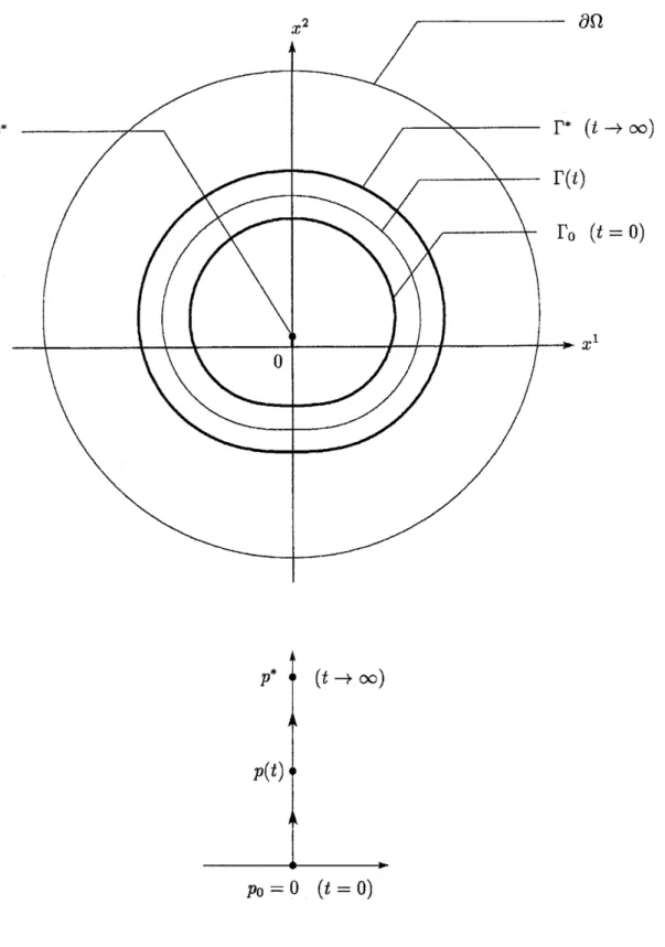
where $r^{*}$ is a constant

(the phaseportrait for (ODE) is as FIGURE 2). This immediatelyyields that (IE) has

a time global solution $(\Gamma(t), v(t))$ such that $v(t)arrow 0$ and $\Gamma(t)=\mathrm{r}(\mathrm{t})$ aproaches

an

(6)

3 CENTER-OF-MASS follows

Using the

ODE

expression (ODE) for (IE), we can discuss the center-of-mass

motion for the interfaces governed by (IE). For each interface $\Gamma$

,

its center of mass

$p\in \mathbb{R}^{N}$i$\mathrm{s}$ defined by

(3.1) $p:= \frac{1}{|\Gamma|}\int_{\Gamma}xdS_{x}^{\Gamma}$

.

Our question is:

How does the center ofmass $p(t)$ evolve when the interface $\Gamma(t)$ is driven

by the interface equation (IE)?

We work under the following convention for theinitial interface $\Gamma_{0}$:

Whenever an initial interface $\Gamma_{0}$ is given, we identify its center ofmass $p\mathrm{O}$

as the origin $0\in \mathbb{R}^{N}$ by an appropriate translation.

We examine the center of mass $p_{r}$ for the interface $\Gamma_{r}$ instead of$p(t)$ for $\Gamma(t)$ since

the interface $\Gamma(t)$ driven by (IE) is characterized as $\Gamma(t)=\Gamma_{f(\ell\}}$

.

The center of mass

$p_{r}$ is computed, by employing the symbols in

\S 2.1,

as

$p$, $=$ $\frac{1}{|\Gamma_{r}|}\oint_{\Gamma_{f}}xdS_{x^{r}}^{\Gamma}$ $=$ $\frac{1}{g(r)}\int_{\mathrm{A}l}(\varphi(y)+rn(y))dS_{y}^{t}$ $=$ $\frac{1}{g(r)}\int_{\mathcal{M}}(\varphi(y)+rn(y))\sum_{j=0}^{N-1}Hj(y)r^{j}dS_{y}^{0}$ $=$ $\frac{1}{g(r)}\sum_{j=0}^{N-1}[r^{j}\int_{\lambda^{l}\mathrm{t}}Hj(y)\varphi(y)dS_{y}^{0}+r^{j+1}\int_{\lambda 4}Hj(y)n(y)dS_{y}^{0}]$ $=$ $\frac{1}{g(r)}[\int_{\lambda 4}H_{0}(y)\varphi(y)dS_{J}^{0}y+r\int_{\mathcal{M}}H_{0}(y)n(y)dS_{y}^{0}]$ $+ \frac{1}{g(r)}\sum_{\mathrm{i}=1}^{N-1}[r^{j}\int_{\mathrm{A}I}Hj(y)\varphi(y)dS_{y}^{0}+r^{j+1}\oint_{A4}Hj(y)n(y)dS_{y}^{0}]$ $=$ $\frac{1}{g(r)}\sum_{j=1}^{N-1}[r^{j}\int_{\mathrm{A}\mathrm{f}}Hj(y)\varphi(y)dS_{y}^{0}+r^{j+1}\oint_{u}.Hj(y)n(y)dS_{y}^{0}]$

.

The last equality follows from $H_{0}(y)\equiv 1$ (by definition), $\int_{\lambda 4}\mathrm{p}(\mathrm{t})dS_{y}^{0}=p_{0}|\Gamma_{0}|=0$

(by our convention) and $f_{\Lambda 4}n(y)dS_{y}^{0}=0$ (by the Gauss divergence theorem).

Since

$\Gamma(t)$ is expressed as $\Gamma(t)=\Gamma_{\tau(t)}$, we have$p(t)=\mathrm{p}\mathrm{r}(\mathrm{t})$, i.e.,

(7)

This expression, however, israther involvedand the dynamics of$p(t)$ is not clear.

Sowenow examine it undertherestriction $N=2$. In this case, the expression of$p(t)$

above becomes quite simple. Indeed, by employing

$H_{1}(y)=\kappa(y)$ (the curvature ofthe initial curve $\Gamma_{0}$ at $\varphi(y)$),

$g(r)=|\Gamma_{0}|+2\pi r$,

$\int_{\Lambda\Lambda}\kappa(y)n(y)dS_{y}^{0}=0$ (by Frenet’sformula),

we find from (3.2) that the center of mass $p(t)$ for (IE) with $N=2$ is givenby

(3.3) $p(t)=\tau_{0}(r(t))q_{0}$

with

$\tau_{0}(r):=\frac{r}{|\Gamma_{0}|+2\pi r}$,

(3.4)

$q_{0}:= \int_{\mathrm{A}l}\kappa(y)\varphi(y)dS_{y}^{0}\in \mathbb{R}^{2}$

.

Note that $\tau_{0}(0)=0$ and $\tau_{0}’(0)>0$

.

By virtue of the expression as in (3.3) and

the monotonousness of$\tau_{0}(r)$ and $r(t)$-dynamics for (ODE),

we

immediately find the

following:

(i) The initial curve $\Gamma_{0}$ uniquely determines a direction

of center-of-mass

motion

as $q_{0}$ in (3.4).

(ii) Suppose that $v_{0}\neq 0$

.

If}

in addition, $\Gamma_{0}$ is an initial curve satisfying $q\mathit{0}\neq 0$, then

the center

_of

mass

$p(t)$ evolves monotonously in $\pm q_{0}$ direction when $\pm v\mathit{0}>0_{J}$

respectively.

We note that the center of

mass

for $\Gamma(t)$ does not evolve in a situation where

an initial curve $\Gamma_{0}$ satisfies $q_{0}=0$. For instance, in the case where

$\Gamma_{0}$ is a circle

or an ellipse. Such examples

suggest

that the vector $q_{0}$ plays a role as an indicator

measuring how muchthe

symmetry

ofthe initial curve$\Gamma_{0}$ is broken overthewhole of

$\Gamma_{0}$

,

although

no

precise

geometrical

characterization of$q_{0}$ have been obtained.

We

now

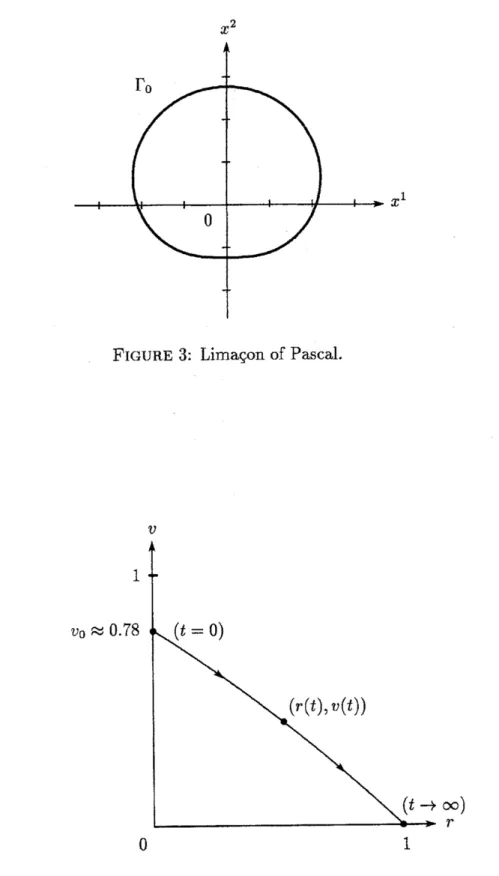
illustratethis aspect by presenting a simple example.

EXAMPLE

3.1

(limagon of Pascal). The curve defined by

$\Gamma_{0}:=\{\varphi(y)=(x^{1}(y), x^{2}(y))|y\in \mathcal{M}=[0,2\pi]\}$

with

$\{$

$x^{1}(y):=\cos y\sin y+2\sin y$

,

(8)

is one ofthe curves calledlimagonof Pascal. The last termon the right hand side of

$x^{2}$-component is added so that _{$p_{0}=0$}, $E$being the usual complete elliptic integralof

2nd kind defined by $E(k^{2}):= \int_{0}^{\pi/2}\sqrt{1-k^{2}\sin^{2}\theta}$dO. By the definition of $q_{0}$ in (3.4),

it yields after some computation that

$q_{0}=(0,$ $\frac{15\pi}{8}-\frac{\pi^{2}}{6E(8/9)})\approx(0, 4.41)$

.

One can see that $q_{0}$, parallel to the

$x^{2}$-axis, precisely coincides with the direction in

which the symmetry of $\Gamma_{0}$ is broken (cf. FIGURE 3). $\square$

Let us now choose $\Gamma_{0}$ above as initial curve and solve the interface equation (IE). To facilitate computation, we employ thefollowing linearfunctions for $h^{\pm}(v)$:

$h^{\pm}(v)=- \frac{1}{2}v\pm 1$,

$-1<v<1$

.

Sincethe center-of-mass motionfor (IE) does not dependon the shape of

an,

wemay

assume, without loss ofgenerality, that $\Omega$ is a disk. We choose and fix the radius so

that $|\Omega|=27\pi\approx$ 84.82, which guarantees that $\Gamma_{0}$ stays uniformly away from

an.

It

turns out that $\Gamma_{0}$ satisfies the following properties:

$|\Gamma_{0}|=12E(8/9)\approx$ 13.36,

$|\Omega_{0}^{-}|=9\pi/2\approx$ 14.14,

$|\Omega_{0}^{+}|=|\Omega|-|\Omega_{0}^{-}|=45\pi/2\approx$

70.68.

We also note that the function $\tau_{0}(r)$ turns out to be

$\tau_{0}(r)=\frac{r}{12E(8/9)+2\pi r}$

.

As an initial value $v_{0}$ for (IE), we choose

(3.5) $v_{0}:= \frac{4(\pi+|\Gamma_{0}|)}{|\Omega|}\approx 0.78$

.

We now solve (ODE) which is equivalent to (IE). Note that $h(v)\equiv-4/|\Omega|$ and

$g(r)=|\Gamma_{0}|+27\mathrm{r}\mathrm{r}$. The relation $dv/dr=h(v)g(r)$ implies that the solution curve in

this situation is given by

$\{(r, v)|v=-\frac{4\pi}{|\Omega|}r^{2}-\frac{4|\Gamma_{0}|}{|\Omega|}r+\frac{4(\pi+|\Gamma_{0}|)}{|\Omega|}|$

.

$r\geq 0$

,

_$v>0\}$

,

which implies the existence ofa globally-in-time solution $(r(t), v(t))$ which converges

to $(1, 0)$ as $tarrow$ oo (cf. FIGURE 4). The center of

mass

$p^{*}$ of the

limit

interface

$\Gamma"=\Gamma_{f}|_{\mathrm{r}=1}$ is given by

$p^{*}=\tau_{0}(1)q_{0}\approx(0,0.22)$.

Therefore,the center of

mass

$p(t)$

,

withtheinitial

curve

$\Gamma_{0}$ being the limagonof Pascal

in EXAMPLE 3.1, evolvesmonotonouly from $(0, 0)$ along the $x^{2}$-axis to

$p^{*}\approx(0,0.22)$

(9)

REFERENCES

[1] N.D. Alikakos, L.Bronserd and G.Fusco, Slow motion in the gradient theory

_of

phase rransitions via energy and spectrum, Calc. Var. Partial Differential

Equa-tions 6 (1998), 39-66.

[2] N. D. Alikakos, X.Chenand G.Fusco, Motion

_of

a droplet by

_surface

tension along

the boundary, Calc. Var. Partial Differential Equations 11 (2000),

233-305.

[3] N. D. Alikakos,

G.

Fusco and G.Karali, Motion

_of

bubbles towards the boundary

for

the

Gahn-Hilliard

equation, European J. Appl. Math. 15 (2004), 103-124.

[4] L. Bronsard and B. Stoth, Volume-preserving mean curvature

_flow

as a limit

_of

$a$

nonlocal Ginzburg-Landau equation, SIAM J. Math. Anal. 28 (1997),

769-807.

[5] J. Escher and G.Simonett, The Volume preserving mean curvature

_flow

near

spheres, Proc. Amer. Math. Soc. 126 (1998),

2789-2796.

[6] M.Gage, On an area-preserving evolution equation

_for

plane curves, Contemp.

Math. 51 (1986),

51-62.

[7] G.Huisken, The volume preserving

mean

curvature flow, J. Reine Angew. Math.

382 (1987),

35-48.

[8] K. Okada, Intermediate dynamics

_of

internal layers

_for

a nonlocal

reaction-diffusion

equation, preprint (2004), to appear in Hiroshima Math. J. 35 (2005).

[9] J. Rubinstein and P.Sternberg, Nonlocal

_{reaction-diffusion}

equations and

nucle-ation, IMA J. Appl. Math. 48 (1992),

249-264.

[10] K.Sakamoto, Spatial homogenization and internal layers in a

reaction-diffusion

system, Hiroshima Math. J. 30 (2000),

377-402.

[11] M.J. Ward, Metastable bubble solutions

_for

the Allen-Cahn equation with mass

conservation,

SIAM

J. Appl. Math. 56 (1996),

1247-1279.

[12] M. J.Ward, The dynamics

of

localized solutions

of

nonlocal

reaction-diffusion

(10)

FIGURE

FIGURE 1: Interface $\Gamma$ and subdomains $\Omega^{\pm}$ in $\Omega$.

$v$

$r$

(11)

$x^{2}$

$x^{1}$

FIGURE 3: Limac.on of Pascal.

$v$ 1 $v_{0}\approx 0.78$ $\infty)$ $r$

01

(12)

$p_{0}=0$ (t $=0)$