Discrete Optimal Testing/Maintenance Policy in a Software Development Project (Decision Theory and Optimization Algorithms)

Discrete

Optimal

Testing/Maintenance Policy

in

a

Software

Development

Project

林坂弘一郎

,

土肥正

Koichiro

Rinsaka and

Tadashi

Dohi

Department

of Information Engineering,

Graduate

School of Engineering,

Hiroshima

University,

Japan

1

Introduction

It is importantto determine the optimal timewhen software testing should be stopped and when the

systemshouldbedelivered to

a user or a

market. Thisproblem,called optimal

_softw

are

releaseproblem,

plays

a

central role for the

success or

failure of

a

software development project. Okumoto and Goel [1]

assumed thatthe number ofsoftware faults detected inthetestingphase isdescribed by

an

exponential software reliability model based

on

a

non-homogeneous Poisson process (NHPP) [2], and derived

an

optimal software release time which minimizes the total expected software cost. Koch and Kubat [3]

considered thesimilar problemfor the othersoftware reliabilitymodel byJelinski and Moranda [4]. Bai

and Yun [5] calculated the optimal number of faults detected before the releaseunder theJelinski and

Moranda model. Many authors formulated the optimal software release problems based on different

model assumptions$\mathrm{a}\mathrm{n}\mathrm{d}/\mathrm{o}\mathrm{r}$several software reliability models $[6, 7]$

.

It isdifficult to detect and

remove

allfaults remaining in

a

software during the actual testing phase,

because exhaustive testing of allexecutablepathsina generalprogramis impossible. Oncethesoftware

is released tousers, howeverthesoftware failures may

occur

even

intheoperational phase. It is

common

for softwaredevelopers to provide maintenanceservice duringthe period when they

are

still responsible

for fixing softwarefaults causing failures. In order tocarryout the maintenance in the operationalphase,

the software developer has to keep

a

software maintenance team. At the

same

time, the management

cost in the operationalphase should be reduced

as

much as possible, but at the

same

time the human

resources

should be utilized effectively. Although the problem which determines themaintenance period

is importantfromthe practical pointofview, onlya veryfew authors paid their attentionto thisproblem.

Kimura et al. [8] considered the optimal software release problem in the

case

where the software

warranty period is

a

random variable. Pham and Zhang [9] developed

a

software cost model with both

warranty and risk. They focused on the problem for determining when to stop the software testing

under

a

warrantycontract. However, it isnoted that the software developer has todesign the warranty

contract itself andoften provides the posterior service for

users

after software failures. Dohi et al. [10]

formulated theproblemfor determining the optimalsoftwarewarranty period whichminimizes the total

expected softwarecostunder the assumption that the debugging processinthe testing phase isdescribed

by

an

NHPP. SandohandRinsaka [11] considered the design problem of

a

maintenanceservicecontract

by regarding

as

the Stackelberg game between

a

software agent and

a

software

user.

Since the user’s

operational environment is not always

same as

thatassumed in the software development phase, however,

theabove literature did not take account

of

the difference between two different phases.

Several reliability assessment methods during the operational phase have been proposed by

some

authors $[12, 13]$

.

_{Rinsaka and Dohi [14] developed}

a

continuous time model for designing the optimal

testingandmaintenance periods, wherethedifference between the software testingenvironmentand the

operational environment

are

reflected.

In thispaper,

we

focus onthe optimalsoftware $\mathrm{t}\mathrm{e}\mathrm{s}\mathrm{t}\mathrm{i}\mathrm{n}\mathrm{g}/\mathrm{m}\mathrm{a}\mathrm{i}\mathrm{n}\mathrm{t}\mathrm{e}\mathrm{n}\mathrm{a}\mathrm{n}\mathrm{c}\mathrm{e}$ problem considered in Rinsaka

andDohi [14], and developastochastic model in discretecircumstance,where the difference between the

software testing environment and the operational environmentcan be characterized by

an

environment

factor (see Okamura et al. [13]). More precisely, the total expected software cost is formulated viathe discrete NHPP type of software reliability models [16, 17, 18]. In the special

case

with the geometric fault-detectiontime distribution,

we

derive analytically the optimal testing period (release time) which

minimizesthetotal expected software costunder

a

milder condition. We call the time lengthto complete

the operational maintenance

after

the release

a

planned maintenance limit, and also derive the optimal

plannedmaintenance limit which minimizesthe total expectedsoftwarecost. Innumerical examples with

real data,

we

calculate numerically the joint optimal $\mathrm{t}\mathrm{e}\mathrm{s}\mathrm{t}\mathrm{i}\mathrm{n}\mathrm{g}/\mathrm{m}\mathrm{a}\mathrm{i}\mathrm{n}\mathrm{t}\mathrm{e}\mathrm{n}\mathrm{a}\mathrm{n}\mathrm{c}\mathrm{e}$ policy, combined by testing

periodand plannedmaintenance limit.

2

Model

Description

First,

we

$\mathrm{m}$ake the following assumptions

on

the software fault-detection process:

(a) In eachtime when

a

software failureoccurs, thesoftware fault causing the failure

can

be detected

and removed immediately.

(b) The number ofinitial faults contained in the software program, $N_{0}$, is given by the Poisson

dis-tributed random variable withmean $\mathrm{i}$ $(>0)$

.

(c) The timeto detect eachsoftware fault is independent and identicallydistributed nonnegative

dis-creterandom variable with probability

mass

function$p_{i}$ $(i= 0, 1, 2, \cdots)$and probability distribution

function$P(i)= \sum_{k=1}^{i}p_{k}$, where$0\leq p_{l}\leq 1$ and$0\leq$ P(i) $\leq 1.$

Let $\{N_{i}, i=1,2, \cdots\}$

be

the cumulative number of

software

faults detected up to time $i$

.

From the

aboveassumptions, the probability

mass

function of$N_{i}$ is given by

Pr$\{N_{i}=ml\}$ $=$ $\frac{\{\omega\sum_{k_{-}^{-}1}^{i}p_{k}\}^{m}}{m!}e^{-\omega\sum_{k=1}\mathrm{p}k}\dot{.}$

$=$ $\frac{\{\omega P(i)\}^{m}}{m!}e^{-\omega P(i)}$ $m=0,1,2$,$\cdots$

.

(1)

Hence, thestochastic process $\{N_{i}, i=1,2, \cdots\}$is equivalent to

a

discrete time NHPPwith

mean

value

function$\omega P(i)$

.

Suppose that

a

softwaretesting is started at time$i=0$ andterminated at time $i=n_{0}(\geq 0)$

.

After

completing the software testing, the software product is released toa

user or

the market. The time length

ofsoftware life cycle $n_{L}(>0)$ is a known constant in advance and is assumed to be sufficiently larger

than $n_{0}$. More precisely, the software life cycle is measured from the point of time $n_{0}$

.

The software

developer isresponsible tothe maintenance serviceforall thesoftware failuresthatmay

occur

duringthe

software lifecycle under

a

maintenancecontract. We suppose thatthe projectmanager decides to break up the maintenance team at time $n_{0}+$ $tty$ for reduction of the operational costto keep it, btit

a

large

amount of debuggingcost during $(n_{0}+nW, n_{0}+n_{L}]$ may be needed if the software failure

occurs.

Let

$n_{W}$ be the planned

maintenance

limit denoting thetime length to complete theoperationalmaintenance

after the release aplanned maintenance limit. Further,

we

definethe following cost components

$\mathrm{c}0$ $(>0)$: cost to

remove

each fault inthe testing phase,

$cw(>0)$: cost to

remove

each fault before the planned maintenancelimit,

$c_{L}(>0)$: cost to

remove

each fault afterthe plannedmaintenance limit,

$k0(>0)$: testing cost per unit oftime,

$k_{W}(>0)$: operationalcost

to

keep themaintenance team per unit oftime.

In thefollowingsection, weformulate the totalexpectedsoftware cost by introducing the above cost

factors

in testing and operational phases. We derive the discreteoptimal software testing period$n_{0}^{*}$

or

the discrete optimal planned maintenancelimit $n_{W}^{*}$ whichminimizes thetotal expectedsoftware cost at

the end ofthe software life cycle. Then, we calculate the joint optimal policy $(n_{0}^{**}, n_{W}^{**})$ combined by

bothtesting period and planned maintenance limit.

3

Total Expected

Software Cost

We formulate the total expected software cost which

can

occur

inboth testingand operational phases.

In theoperationalphase,

we

considertwo cost factors; the maintenancecost due to the software failure

and the operationalcostto keep the maintenance team.

From Eq.(l), the probability

mass

function ofthe number of software faults detected during the

It should be noted that the operational environment after the release may differ from the

debug-ging environment in the testing phase. This difference is similar to that between the accelerated life

testing environment and the normal operating environment for hardware products. We introduce the

environment factor $a(>0)$ which represents the relative severity in the operational environment after

the release, andassumethat the timesinthe testingphaseand the operational phase have aproportional

relationship. Namely, the time length $n$ in the operational phase corresponds to $a\cross n$ in the testing

phase. Under the above assumption, $a=1$

means

the equivalence between the testing andoperational

environments.

On

the other hand,

$a>1(a<1)$

implies that the operational environment is

severer

(looser)thanthe testingenvironment. Okamura et $al$ $[13]$ apply this techniquetomodel the operational

phase ofthe software, and

estimate

the software reliability through

an

example in the actual software

development roject. The probability

mass

functionofthenumber of software faults detected beforethe

planned maintenance limit is given by

$\mathrm{P}\mathrm{r}\{N_{n\mathrm{o}+n_{W}}-N_{n_{0}}=m\}=\frac{\{\omega\{P(n_{0}+[an_{W}])-P(n_{0})\}\}^{m}}{m!}e^{-\omega\{P(n_{0}+[an_{W}])-P(n\mathrm{o})\}}$, (3)

where, $[\cdot]$ is the Gaussianinteger.

Similarly,thefault-detection process of the software after the planned maintenance limit is expressed

by

$\mathrm{P}\mathrm{r}\{N_{n_{0}+n_{L}}-N_{n_{0}+n_{W}}=m\}$

$=$ $\frac{\{\omega\{P(n_{0}+[an_{L}])-P(n_{0}+[an_{W}])\}\}^{m}}{m!}e^{-\mathfrak{l}d}\{P(\mathrm{y}\mathrm{r}_{0}+[a\mathrm{v}\mathrm{z}_{L}])-P(n\mathrm{o}+[an_{W}]\rangle\}$

.

(4)

From Eqs.(2), (3) and (4), thetotal expected software cost isgiven by

$C(n_{0}, n_{W})$ $=$ $\mathrm{k}\mathrm{o}\mathrm{n}\mathrm{o}+$$cou)P(no)+kwnw$ _{$+c_{W}\omega$$\{P(n0+[anw])- P(\mathrm{n}\mathrm{o})\}$}

1-$c_{L}\omega\{P(n_{0}1-[an_{L}])-P(n_{0}+[anw])\}$

.

(5)

4

Determination of the

Optimal

Policies

In thissection

we

derive the optimal testing period $n_{0}^{*}$ orthe optimal planned maintenance limit $n_{W}^{*}$

whichminimizesthetotal expected software cost incurred to thesoftwaredeveloper at the end of software

life cycle. Suppose thatthe time to detect each software fault obeysthe geometric distribution

$p_{i}=b(1-b)^{i-1}$ (6)

with parameter$b(0<b<1)$

.

In this case, the totalexpectedsoftware cost inEq.(5) becomes

$C(n_{0}, n_{W})$ $=$ $k_{0}n_{0}+c_{0}\omega\{1-(1-b)^{n0}\}$$+kwnw$$+c_{W}\omega\{(1-b)^{n_{0}}-(1-b)^{n_{\mathrm{O}}+[an_{W}]}\}$

$+c_{L}\mathrm{u}$$\{(1-b)^{n_{0}+[an_{W}]}-(1-b)^{n_{\mathrm{O}}+[an_{L}]\}}$

.

(7)

We makethe following assumptions:

(A-I) $a$ is positive and an integer value,

(A-II) $c_{L}>cw$ $>c_{0}$,

(A-III) $c_{W}\{1-(1-b)^{an_{L}}\}>c_{0}$,

(A-IV) $c_{W}\{1-(1-b)^{an_{W}}\}+c_{L}\{(1-b)^{an_{W}}-(1-b)^{an_{L}}\}>$ _c0.

Define

$Q(nw)=k_{0}+\omega b\{c_{0}-c_{W}(1-(1-b)^{an_{W}})-c_{L}((1-b)^{anw}-(1-b)^{an_{L}})\}$

.

(8)

Then the following result provides the optimalsoftwaretesting policywhich minimizesthe total expected

Theorem 1: When the $sof$ _tware

fault-detection

time distribution

follows

the geometric

distribution

withparameter$b(0<b<1)$, under the assumptions (A-I) to (A-IV), the optimal$sof$rware testingperiod

(release time) which minimizes the total expected

_software

cost is given as

_follows:

(1)

_If

$Q(nW)<0,$ then there exist (at least one, at most two)

_finite

optimal

_software

testing periods

(release times)$n_{0}^{*}(>0)$

.

(2)

_If

$Q(n_{W})\geq 0,$ then the optimal policy is$n_{0}^{*}=0$ with

$\mathrm{C}(\mathrm{n}0, n_{W})=kwnw$ $+c_{W}\omega\{1-(1-b)^{an_{W}}\}+cL\omega\{(1-b)^{an_{W}}-(1-b)^{an_{L}}\}$

.

(9)

Furthermore, the following result provides the optimal planned maintenance limit which minimizes

the total expected software cost.

Theorem 2: When the

_{software fault-detection}

time distribution

_follows

the geometric distribution

with parameter$b(0<b<1)$

,

underthe assumptions (A-I) and (A-II); the optimal planned maintenance

lirnit which minimizes the total expected

_software

cost is given

as

_follows:

(1)

_If

$k_{W}\geq$ ($c_{L}-$cw)u{1--(1-b)a} $(1-b)^{n_{0}}$, then the optimalpolicy is$n_{W}^{*}=0$ with

$\mathrm{C}(\mathrm{n}0, n_{W}^{*})=$konQ$+c_{0}\omega$

{

$1-(1-$

b)a}$+c_{W}\omega\{(1-b)^{n_{0}}-(1-b)^{n_{0}+an_{L}}\}$

.

(10)

(2)

_If

$k_{W}<(\mathrm{c}_{L} \mathrm{c}\mathrm{w})\mathrm{u}$

{

$1-(1-$

b)a}$(1-b)^{n0}$ and_{$k_{W}>$} (_{$c_{L}-$}cw)u{1--(1-b)a}$(1-b)^{n_{0}+a(n_{L}-1)}$,

then thereexist (at least one,

at

most two) optimal plannedmaintenance limits$n_{W}^{*}(0<n_{W}^{*}<n_{L})$

which minimizes the total expected

_software

cost.

(3)

_If

$k_{W}\leq$ (_{$c_{L}-$}cw)u{1--(1-b)a} $(1-b)^{n\mathrm{o}+a(n_{L}-1)}$, then

we

have _{$n_{W}^{*}=nL$} with

$\mathrm{C}(\mathrm{n}0, \mathrm{n}\mathrm{w})=\mathrm{k}\mathrm{o}\mathrm{n}\mathrm{Q}+c_{0}\omega$

{

$1-(1-$b)a}

-lJcw

$n_{L}+cw\omega\{(1-b)^{n_{0}}-(1-b)^{n_{0}+an_{L}}\}$

.

(11)

5

Numerical

Examples

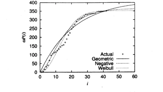
Basedon 351 softwarefault(41 week) data observed in the realsoftware testing process [19],wecalculate

numerically the optimal testing period$n_{0}^{*}$and the optimal planned maintenance limit$n_{W}^{*}$ whichminimize

the total expected software cost. Further, we compute the joint optimal policy $(n_{0}^{**}, n_{W}^{**})$ minimizing

$C(n_{0}, n_{W})$. Forthe software fault-detectiontime distribution,

we

apply three probability distributions;

geometric, negative binomial and discrete Weibull distributions. The probability

mass functions

for

negative binomial and discrete Weibull

are

given by

$p_{i}=($ $h+h$$\mathrm{z}$$-21$

)

$b^{h}(1-b)^{i-1}$, (12)

and

$p_{i}=b\dot{\cdot}h-b^{(\mathrm{z}+1)^{h}}$ (13)

respectively, where$h\geq 0.$ Fornegativebinomial and discrete Weibull distributions,

we

considerthe

case

of$h=2.$

Suppose that the unknown parameters in thesoftwarereliability models

are

estimatedbythemethod

of maximum likelihood. Then,

we

have the estimates $(\hat{\omega},\hat{b})=$ (413.305, 0.0451012) for the geometric

model, $(\hat{\omega},\hat{b})=$ (364.234, 0.116255) for the negative binomial model and $(\hat{\omega},\hat{b})=$ (351.871, 0.996436)

for the discrete Weibull model. Figure 1 shows the actual software fault data and the behavior of

estimated

mean

value functions.

Since

the environment factor$a$ is

a

subjective parameterwhichshould

be estimated from thepast development track record,

we

assume

thatthe value of$a$ is known. For the

other model parameters,

we assume:

$k_{0}=2.0,$ $k_{W}=1.0$, $c_{0}=5.0$, $c_{W}=10.0$

,

$c_{L}=50.0$and $n_{L}=200.$

Table 1 presents the dependence ofenvironment factor $a$

on

the optimal testing period $n_{0}^{*}$ when $nW=20.$ Asthe environment factor monotonically increases, $i.e$

.,

the operational circumstance tends

tobesevere,itisobserved that the optimal testing period$n_{0}^{*}$ and itsassociatedminimum total expected

software cost $C(n_{0}^{*}, 20)$ decrease for both geometric and negative binomial models. For the discrete

5

400

350

\sim .--.---.---,

300

$.’\dotplus,\dotplus,,\cdot.\dotplus^{\dotplus,’},\sim$ $.j^{j’}$.

250

$\vee\wedge-$

’.’

$\ell+$

200

$\mathrm{e}$ $\prime\prime\prime.’.\cdot+’+$

150

$l^{J’}.\dotplus^{+}\cdot$ $!’$

$\mathrm{i}00$ $,+.\cdot’$

.

Actual

$+$

Geometric

–

50

Ne

ative

– $,.*\prime\prime,+.\cdot$

.

eibull

$\ldots.----$

00

$\mathrm{i}0$

20

40

50

$i$

Figure 1: Behavior ofactualsoftware fault data and estimated

mean

value functions.

Table 1: Optimal software testing period for varyingenvironment factor.

Geometric Negative Weibull

a $n_{0}^{*}$ $C(n_{0}^{*}, 20)$ $n_{0}^{*}$ $C(n_{0}^{*}, 20)$ $n_{0}^{*}$ $C(n_{0}^{*}, 20)$ 0.50 122 2375 65 1990 41 1867 0.75 119 2367 62 1983 40 1865

1.00

115 2359 59

1977

39 1865 1.25 111 2352 57

1973

39

1865

1.50

$10\underline{8}$ 2345 56

1971

39 1865

2.00

101

2333

54

1967

39

1865

3.00

93

2315 53

1966

39

1865

Table 2: Optimal planned maintenance limit for varying environment factor.

Geometric Negative Weibull

a $nW$ $\mathrm{C}(41,\mathrm{n}\mathrm{f}\mathrm{c})$ $n_{W}^{*}-$ _{$C(41, n_{W}^{*})$} $n_{W}^{*}$ $C(41,n_{W}^{*})$ 0.50

176

2648 62 2050 12

1863

0.75

128

2615

48 2028

81859

1.00

103 $\overline{2584}$

38

2016

81856

1.25 88

2564

32

2008

81855

1.50

74 2549 28

2003

61854

2.00

59

2530 22 1996

51852

3.00 42 2509 16 1988 41850

Table 3: Optimaltesting$\mathrm{p}\mathrm{e}\mathrm{r}\mathrm{i}\mathrm{o}\mathrm{d}/\mathrm{p}\mathrm{l}\mathrm{a}\mathrm{n}\mathrm{n}\mathrm{e}\mathrm{d}$maintenancelimit for varyingenvironment factor.

Geometric Neg tive Weibull

a $n_{()}^{*}$ $n_{W}^{**}$ $C(\circ**,n_{W}^{**})$ $\overline{n_{0}^{**}}n_{lV}^{**}-$ $C(n_{0}^{**},n_{W}^{**})$ $0**$ $n_{W}^{**}$ $C(n_{0}^{**}, W**)$ $0$

.

0 131 0 2372 3 0 1986 47 0 1859

0.75

108 40 236 64 16 1983 42

-8

1858 1.00 99 4 23 260

-19

1977

42 7 1856 1.25 94 44 2343 57 20

1973

41 8 1855 1.50

93

40

2335

57

16

1970

41 6

1854

2.00

90 34 2324

56

14 1966 41 5 1852

3.00

88

27

2312 55 11 1960 40 4 1850

in Fig.1, it is observed that the optimal testing period is strongly influenced byvarying environment factor.

Table2showsthedependenceof environment factor$a$on theoptimalplanned maintenance limit$n_{W}^{*}$

in

case

of$n_{0}=41.$ It is found that the optimal planned maintenance limit $n_{W}^{*}$ and the corresponding

minimum total expected software cost $C(41, n_{W}^{*})$ decrease

as

the environment factor monotonically

increases. Thistendency

can

be explained as follows: The residual faults insoftware

are

detected and

removedatthe early stageintheoperational phase

as

theoperationalenvironment becomes

more severe.

Then, the possibility that the software failure

occurs

in the latter stage of the operational phase

may

become small. Hence, the implication in which the software developer keeps the maintenance team becomes smaller towardthe end of the life cycle.

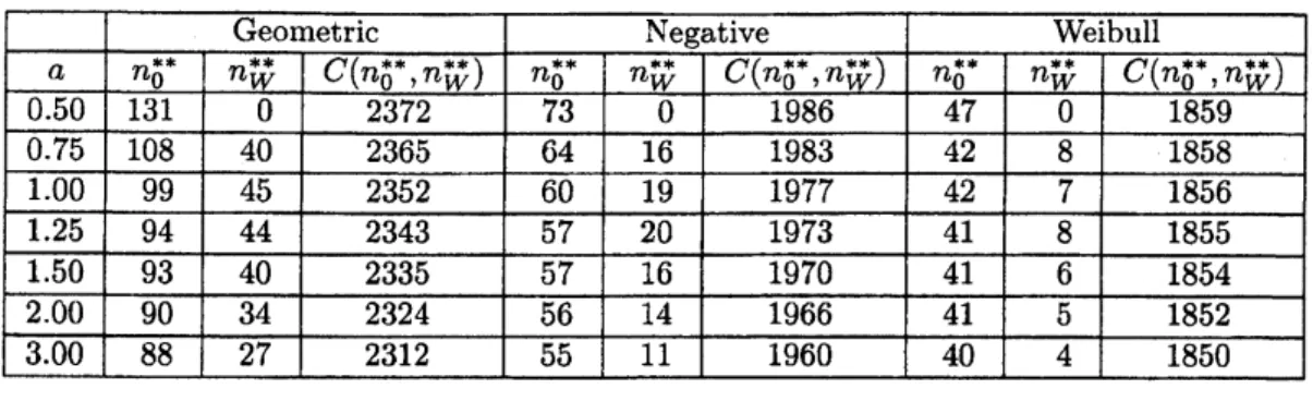
Table 3 examines the dependence of environment factor $a$

on

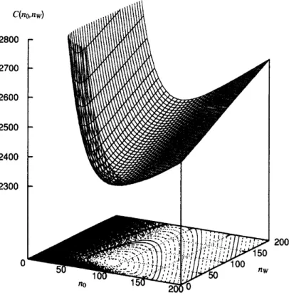
the joint optimal policy $(n_{0}^{**}, n_{W}^{**})$

combined by testing period and planned maintenance limit. Figure 2 illustrates the behavior ofthe

expected cost for the geometric model when $a=$ 2.00. It is observed from Table 3 that the optimal

testing period $n_{0}^{**}$ decreases

as

theenvironment factor monotonically increases, but, the monotonicity

ofthe optimal planned maintenance limit $n_{W}^{**}$ is not observed. It is also

seen

that the minimum total

expectedsoftware cost $C(n_{0}^{**}, n_{W}^{**})$ decreases

as

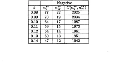
the environment factormonotonically increases.

Tables 4, 5 and 6 present the dependence ofthe software reliability model parameter $b$

on

the joint

optimal policy $(n_{0}^{**}, n_{W}^{**})$

.

It is observed that the optimal testing time, optimal planned maintenance

limit and its associated minimum total expectedsoftware cost decrease asthe fault detection becomes easier.

6

Concluding Remarks

In this paper,

we

have assumed that the software developer

was

responsible tothe

maintenance service

for all the software failures that

occur

during the software lifecycle under the

maintenance

contract. In order to carry out the maintenance service in the operational phase, thesoftware developer has to keep

a

software maintenance team. At the

same

time, themanagement cost in the operationalphase has to

be reducedas much

as

possible, but human

resources

should be utilized effectively. We have called the time length to complete the operational maintenance after the release the planned maintenance limit,

and have controlled it in terms ofcost-benefit analysis. We have developed the discrete model which

represents the difference in the software execution environment during testing and operational phases,

using the

same

method

as

the continuous-time-based reliability assessment modeling in the operational

phase proposed by

Okamura

et $al$ $[13]$

.

Based

on

the discrete NHPP

we

have

formulated

the total

expected software cost incurred tothe software developer at the end of softwarelife cycle. The optimal

testingperiod (release time) andoptimal planned maintenance limit which minimize the totalexpected

software

cost have been

derived.

Then, throughout the numerical examples,

we

have discussed the joint

Table 4: Optimal testing period$/\mathrm{p}\mathrm{l}\mathrm{a}\mathrm{n}\mathrm{n}\mathrm{e}\mathrm{d}$ maintenance limit for geometricsoftwarereliability model with varying parameter b. $\mathrm{G}\overline{\mathrm{e}\mathrm{o}}\mathrm{m}\mathrm{e}\mathrm{t}\mathrm{r}\mathrm{i}\mathrm{c}$ $b$ $n_{0}^{**}$ $n_{W}^{**}$ $C(n_{0}^{**},n^{**})$

0.042

37

2340 0.043 36

2335

0.044 35 2330

0.045

35

2325

0.046 34 2320

0.047

33 2315 0.048 32 2311

Table

5:

Optimal testing $\mathrm{p}\mathrm{e}\mathrm{r}\mathrm{i}\mathrm{o}\mathrm{d}/\mathrm{p}\mathrm{l}\mathrm{a}\mathrm{n}\mathrm{n}\mathrm{e}\mathrm{d}$maintenance limit for negative binomial software reliability

model with varying parameter$b$

.

Negative $b$ $n_{0}^{**}$ $n_{W}^{**}$ $C(n_{0}^{**}, n_{W}^{**})$ 0.08

77

22 2025 0.09 70 19 2004 0.10 64 17 1987 0.11 59 15 1973 0.12 54 14

1961

0.13 50 13 1951 0.14 47 12 1942

Table6: Optimal testing$\mathrm{p}\mathrm{e}\mathrm{r}\mathrm{i}\mathrm{o}\mathrm{d}/\mathrm{p}\mathrm{l}\mathrm{a}\mathrm{n}\mathrm{n}\mathrm{e}\mathrm{d}$maintenancelimitfordiscreteWeibull softwarereliabilitymodel

with varying parameter$b$

.

Weibull $b$ $n_{0}^{**}$ $n_{W}^{**}$ $C(n_{0}^{**}, n_{W}^{**})$ 0.999 10

1926

0.998

7 1880 0.997 6

-1880

0.996

5

1847

0.996

4

1838

0.994 4 1832 0.998 4

1827

8

Figure2: Behavior of thetotalexpectedsoftwarecost forgeometric software reliability model$(a=2.00)$

.

References

[1] K. Okumoto andL. Goel, “Optimumrelease timefor softwaresystemsbased onreliability and cost

criteria,” J. Sys. Software, vol. 1, pp. 315-318, 1980.

[2] A.L. Goel and K. Okumoto, “Time-dependent error-detection rate model for software reliability andother performance measures,” IEEE Trans. Reliab., vol. R-28,

no.

3, pp. 206-211, 1979.

[3] H.S. Kochand P. Kubat, “Optimal release time ofcomputersoftware,” IEEE Trans. Software Eng., vol.

SE

9,

no.

3,

pp.

323-327,

1983.

[4] Z. Jelinski and P.B. Moranda, “Software reliability research,” Statistical Computer Performance

Evaluation, (W. Freiberger ed.), pp. $465\triangleleft 84$

,

Academic Press, New York,

1972.

[5] D.S. Bai

and

W.Y. Yun, “Optimum number of

errors

corrected beforereleasing

a

softwaresystem,”

IEEETrans. Reliab., vol. R-37,

no.

1, pp. 41-44, 1988.

[6] W.Y. Yun and D.S. Bai, “Optimum software release policy with random life cycle,” IEEE Trans.

Reliab.,vol. R-39,

no.

2, pp. 167-170, 1990.

[7] T. Dohi, N. Kaioand S. Osaki, “Optimalsoftwarerelease policies withdebuggingtimelag,” Int. J.

Reliab., Quality and Safety Eng., vol. 4,

no.

3, pp. 241-255, 1997.

[8] M. Kimura, T. Toyota and S. Yamada, “Economic analysisofsoftware release problems with

war-ranty costand reliability requirement,”

Reliab.

Eng.

&

Sys. Safe., vol. 66,

no.

1, pp. 49-55,

1999.

[9] H. Pham and X. Zhang, “A

software

cost model withwarrantyand risk costs,” IEEE Trans.

Com-put., vol.48,

no.

1,

pp.

71-75,

1999.

[10] T. Dohi, H. Okamura, N. Kaio and S. Osaki, “The age-dependent optimal warranty policy and

its

application to software maintenance contract,” Proc. 5th Int’l Conf. on Probab. Safe. Assess, _and

9

[11] H. Sandoh and K. Rinsaka, “Maintenance service contract model for software,” Proc. of the First

Western Pacific and Third Australia-Japan Workshopon Stochastic Models in Engineering,

Tech-nology and Management, Christchurch, New Zealand, pp. 466-475, 1999.

[12] J. Musa, G. Fuoco, N. Irving, D. Kropfl and B. Juhlin, “The operational profile,” Handbook of

SoftwareReliability Engineering, (M.R. Lyu ed.), pp. 167-216, McGraw-Hill, New York, 1995.

[13] H. Okamura,T. Dohiand

S.

Osaki, “A reliabilityassessment method for software productsin

oper-ational phase – proposalof

an

accelerated life testingmodel –,” Electronics and Communication

in Japan, Part 3, vol. 84, pp. 25-33,

2001.

[14] K. Rinsaka andT. Dohi, “Optimal$\mathrm{t}\mathrm{e}\mathrm{s}\mathrm{t}\mathrm{i}\mathrm{n}\mathrm{g}/\mathrm{m}\mathrm{a}\mathrm{i}\mathrm{n}\mathrm{t}\mathrm{e}\mathrm{n}\mathrm{a}\mathrm{n}\mathrm{c}\mathrm{e}$ design ina software developmentproject,”

Electronic Proc. of Fourth International Conference

on

Mathematical Methods in Reliability

-Methodology and Practice, Santa Fe, New Mexico, USA, 2004.

[15] A.A. Abde-Ghaly, P.Y. Chan and B. Littlewood, “Evaluation of competing software reliability

predictions,” IEEE Trans. SoftwareEng., vol. SE-12,

no.

9, pp. 950-967, 1986.

[16] S. Yamada and S. Osaki, “Discrete software reliabilitygrowth models,” Applied Stochastic Models

and Data Analysis, vol. 1, pp. 65-77, 1985.

[17] T. Kitaoka, S. Yamada and S. Osaki, “Adiscrete non-homogeneous

error

detection rate model for

software reliability,” Transactions of the Institute of Electronics and

Communication

Engineersof Japan, vol. E69, pp. 859-865,

1986.

[18] H. Okamura, A. Murayama andT. Dohi, “EMAlgorithm for$\mathrm{d}\mathrm{i}\mathrm{s}$-crete softwarereliability models:

a

unifiedparameter estimation method,” Proceedingsof8th IEEE International Symposium

on

High Assurance Systems Engineering, pp. 219-228.IEEE CS Press, 2004.

[19] A.P. Nikora and M. R. Lyu, “Softwarereliabilitymeasurement experience,” Handbook ofSoftware