A computer-assisted study of the Landau-Nakanishi geometry (Recent development of microlocal analysis and asymptotic analysis)

A

computer-assisted

study

of the

Landau-Nakanishi geometry

By

Naofumi

HONDA*

and

Takahiro

KAWAI**

\S 1.

Introduction

The purpose of this article is to call forth the interest of specialists in microlocal

analysis in the computer-assisted study ofthe Landau-Nakanishi geometry by showing

concrete examples whichwe haveencountered inmaking the effort with Henry P. Stapp

to elucidate the concrete contents of Sato’s postulate ([2]) on the analytic structure of the $S$-matrix near the 3-particle threshold. For the convenience of the reader we first

recall the definition ofa Feynman graph$G$and the Landau-Nakanishi variety (hereafter

abbreviated as

en

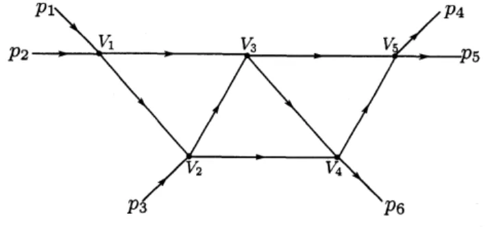
variety) $\mathscr{L}(G)$ associated with $G.$

Definition 1.1. AFeynman graph $G$is

a

graph that consists of finitely many points

$V_{1},$ $V_{2},$

$\ldots,$ $V_{n’}$ (called vertices), finitely many line segments $L_{1},$ $L_{2},$ $\ldots$, $L_{N}$ (called

internal lines) and finitely many half-lines $L_{1}^{e},$ $L_{2}^{e},$

$\ldots,$ $L_{n}^{e}$ (called external lines), where

each of the end-points $W_{\ell}^{+}$ and $W_{\ell}^{-}$ of $L_{\ell}(\ell=1,2, \ldots, N)$ coincides with some $V_{j}$

$(j=1,2, \ldots, n’)$ satisfying the condition

(1.1) $W_{\ell}^{+}\neq W_{\ell}^{-},$

and the (unique) end-point of$L_{r}^{e}(r=1, \ldots, n)$ coincides with some $V_{j}(j=1, \ldots, n’)$

.

In this article we assume that each internal line and each external line are oriented

(and specified with an arrow like – if necessary). Using this orientation we define

the incidence number $b$ : $\ell$] for

a

pair of

a

vertex

$V_{j}$ and

an

internal line $L_{\ell}$ by the

following rule:

(1.2) $[j:\ell]=\{\begin{array}{ll}+1 when the internal line L_{\ell} ends at the vertex V_{j},-1 when L_{\ell} starts from V_{j},0 neither of the end- points of L_{\ell} coincides with V_{j}.\end{array}$

2010Mathematics Subject Classification(s): Primary$81Q30$; Secondary $32S40.$

Key Words: Landau-Nakanishi geometry, Feynmangraph, truss-bridge graph, 3-particlethreshold

*Department ofMathematics, Faculty of Science, Hokkaido University, Sapporo, 060-0810, Japan.

NAOFUMI HONDA AND TAKAHIRO KAWAI

The incidence number $[j:r]$ _{for a pair ofa vertex} $V_{j}$ and an externalline $L_{r}^{e}$ is defined in a similar

manner.

We also assume that a $v$-dimensional real (or complex if so specified) vector _{$p_{r}=$}

$(p_{r,0}, \ldots, p_{r,\nu-1})(r=1,2, \ldots, n)$ is assigned to each external line $L_{r}^{e}$ and a strictly

positive number $m_{\ell}(\ell=1,2, \ldots, N)$ is assigned to each internal hne $L_{\ell}.$

Figure 1. An exampleofa Feynman graph.

Remark 1.2. In this article we assume, for the sake of simplicity, that all constants

$m_{\ell}$ are the

same

and we denote it by the number _$m$. That is, we consider only the

so-called equal

mass

case.

Remark 1.3. Unless otherwise stated, we assume $v=2$ in what follows. Remark 1.4. In this article we do not assume

(1.3) $p_{r}^{2}(=p_{r,0}^{2}-p_{r,1}^{2})=m^{2}.$

In passing we note that, here and in what follows, for $v$-dimensional vector $k=$

$(k_{0}, k_{1}, \ldots, k_{\nu-1})$ the scalar $k^{2}$ stands for $k_{0}^{2}- \sum_{\rho=1}^{\nu-1}k_{\rho}^{2}.$

In order to write down the defining equation of the $\mathscr{L}\mathscr{N}$ variety, we introduce the

followingnumbers $j^{\pm}(\ell)$ and _$j(r)$ for an internal hne $L_{\ell}$ and an external line $L_{r}^{e}$:

(1.4) $[j^{\pm}(\ell):\ell]=\pm 1,$

(1.5) $[j(r):r]\neq 0.$

Definition 1.5. (i) The Landau-Nakanishi variety $\mathscr{L}(G)$ associated with a

Feyn-man graph$G$is, bydefinition, thetotality of_{$(p, \sqrt{-1}u)$} in$\mathbb{R}^{\nu n}\cross(\sqrt{-1}\mathbb{R}^{\nu n})$ thatsatisfies

the following equations for some $(\alpha_{1}, \ldots, \alpha_{N};k_{1}, \ldots, k_{N};v_{1}, \ldots, v_{n’} ; a)\in \mathbb{R}^{N}\cross \mathbb{R}^{\nu N}\cross$

$\mathbb{R}^{\nu n’}\cross \mathbb{R}^{\nu}$

:

(1.6) $\{\begin{array}{ll}\sum_{r=1}^{n}[j:r]p_{r}+\sum_{\ell=1}^{N}[j:\ell]k_{\ell}=0 (j=1,2, \ldots, n’) ,\alpha_{\ell}(k_{\ell}^{2}-m^{2})=0, k_{\ell,0}>0 (\ell=1,2, \ldots, N) ,v_{j^{+}(\ell)}-v_{j^{-(\ell)}}=\alpha_{\ell}k_{\ell} (\ell=1,2, \ldots, N) ,u_{r}=-[j(r) :r](v_{j(r)}+a) (r=1,2, \ldots, n) .\end{array}$

(ii) If $\alpha_{\ell}\geq 0(\ell=1,2, \ldots, N)$ in (1.6), $\mathscr{L}(G)$ is designated as $\mathscr{L}^{+}(G)$ and called the $positive-\alpha\ovalbox{\tt\small REJECT}$’ variety associated with $G.$

(iii) If $\alpha_{\ell}>0(\ell=1,2, \ldots, N)$, then $\mathscr{L}^{+}(G)$ is designated as $\mathscr{L}^{\oplus}(G)$.

Remark 1.6. (i) Ifwe formally define the Feynman integral$F_{G}(p)$ associated with $G$

by

(1.7) $\int\cdots\int\frac{\acute{\prod_{j=1}^{n}}\delta^{\nu}(\sum_{r=1}^{n}[j:r]p_{r}+\sum_{\ell=1}^{N}[j:\ell]k_{\ell})}{\prod_{\ell=1}^{N}(k_{\ell}^{2}-m^{2}+\sqrt{-1}0)}\prod_{\ell=1}^{N}d^{\nu}k_{\ell},$

then it is known ([2]) that under some moderate conditions $F_{G}(p)$ is well-defined

as

a microfunction and that it is supported by $\mathscr{L}^{+}(G)$. Thus $\mathscr{L}^{+}(G)$ is a variety in $\sqrt{-1}S^{*}\mathbb{R}^{\nu n}$. Denoting by $\pi$ the canonical projection map from $\sqrt{-1}S^{*}\mathbb{R}^{\nu n}$ to $\mathbb{R}^{\nu n},$

we denote $\pi(\mathscr{L}^{+}(G))$ by _$L^{+}(G)$

.

It is also called the $positive-\alpha\ovalbox{\tt\small REJECT}\gamma$ variety. When

we want to emphasize that we are dealing with the object projected down to the base

manifold, we sometimes

use

somewhat $10$ose expression “$(positive-\alpha)LN$

surface”

As

we will show in Section 2 and Section 3, some higher codimensional component of an $LN$ “surface” is ofparticular interest.

(ii) When $F_{G}(p)$ is well-defined, it has the form

(1.8) $f_{G}(p) \delta^{\nu}(\sum_{j,r}[j:r]p_{r})$

.

The vector $a$ in the last equation of (1.6) is a counterpart of the factor $\delta^{\nu}(\sum[j : r]p_{r})$

.

The factor $f_{G}(p)$ is called a Feynman amplitude (or function).

Concerning the concrete figure of $L^{+}(G)$ the book of Eden et al. ([1]) is a good

introduction. Thanks to the progress ofcomputers, mathematicians can now make the

NAOFUMI HONDA AND TAKAHIRO KAWAI

Landau-Nakanishi geometry, if they put sufficiently enough energy and time into the

study of the subject. Actually, as we show in Section 2, the detailed description of

$L^{+}(G)$ gives rise to interesting mathematical problems even for a very _{simple graph $G.$}

Section 3 is devoted to showing what kind of anomalies is observed when $G$ contains

what wecall the non-external vertices. Thestudy ofsuch graphs is not only challenging

but also important in our future study of the analytic structure of the $S$-matrix near

the 3-particle threshold, which will make essential use of the Borel resummation.

\S 2.

$LN$ surface $L(G)$ and its $positive-\alpha$ part $L^{+}(G)$ when $G$ is an ice-cream

cone

graph

As oneof themost basic graphthat is relevant tothe 3-particlethreshold weconsider

the so-called ice-cream cone graph, that is,

Figure 2. The ice-cream cone graph $G_{1}.$

The reason ofour interest in$L^{+}(G_{1})$ is twofold. First, $L^{+}(G_{1})$ touches the 3-particle

threshold $3PT$, and we know ([2], [3])

(2.1) $f_{G_{1}}(p)|_{3PT}=a(p)f_{G_{0}}(p)+b(p)$

holds at ageneric point of$3PT$_, where $a(p)$ and $b(p)$ are holomorphicfunctions and the

graph $G_{0}$ is described in the figure below:

Figure 3. The Feynmangraph $G_{0}.$

Second, ifweconsider apoint$p$where thefollowingconfigurationof Fig. 4 isrealized,

that is, if all internal lines are parallel _{keeping each vertex distinct, then we find}

Figure 4. The configuration ofvectors $v_{j}$’s and $\alpha_{\ell}k_{\ell}’ s.$

(2.2) $p_{4}+p_{5}=2p_{6},$

(2.3) $p_{6}^{2}=m^{2}.$

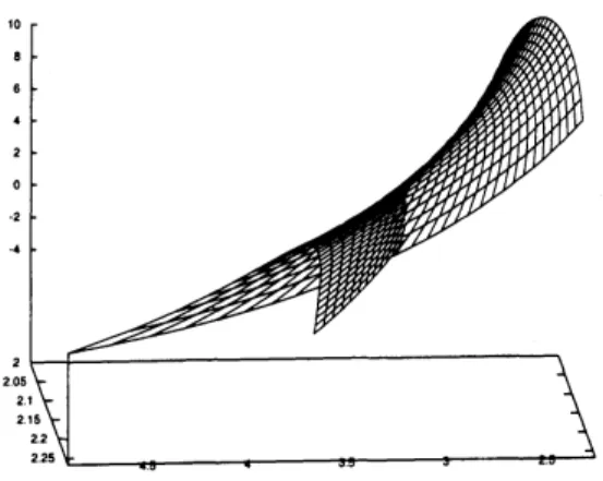
The totality $N_{-}$ of such points covers only a tiny portion of $L^{+}(G_{1})$, but as Fig. 5

showsl

, $N_{-}$ is a crucially important part of the singularity that _{$L^{+}(G_{1})$} presents; the

singularity is commonly known

as

“Whitney’s umbrella”, and $N$-belongs to its most

singular part. Thus explicitly writing down the holonomic system that $f_{G_{1}}(p)$ satisfies

near $N_{-}$ is a charming problem in microlocal analysis.

Figure 5. The “non-zero $\alpha$” $LN$ surface of$G_{1}$ with $\nu=2$ and $m=1.$

lThe surface appearingin the figure is analytically isomorphicto the one defined by the following

equations of parameters $s>0$ and $t>0:x=s+ \frac{1}{s},$ $y= \frac{s^{2}t+3s}{st-1}$ and $z=t$. It has only one

pinch point singularity $N-$ and also has a self-intersection curve corresponding to ashank ofan

NAOFUMI HONDA AND TAKAHIRO KAWAI

\S 3.

Truss-bridge graphs

As our eventual purpose is to understand the analytic structure of the $S$-matrix

near the 3-particle _{threshold, it is natural to try to study the concrete figure of the}

$positive-\alpha$ $LN$ surface $L^{+}(G)$ associated with Feynman graph $G$ when it touches

3-particle threshold. One such a graph is $G_{1}$ studied in Section 2. One can readily note

that $L^{+}(T_{2})$ contains $L^{+}(G_{1})$ and also note that $L^{+}(T_{1})$ touches 3-particle threshold,

where the truss-bridge graph $T_{1}$ (resp. $T_{2}$) is given in Fig. 6 (resp. Fig. 7) below.

Figure 6. The truss-bridge graph $T_{1}$. Figure 7. The truss-bridge graph _{$T_{2}.$}

Thus it is natural to study $L^{+}(T_{3})$, as the next target, where

Figure 8. The truss-bridge graph $T_{3}.$

Interestingly enough, there is no reference which concretely describes $L^{+}(T_{3})$, as far as

we know. And, the actual figure shown in Fig. 9 is highly intriguing; the $LN$ surface

in the figure consists of two irreducible components. One is isomorphic to the surface defined by the following equations of parameters $\mathcal{S}>0$ and $t>0$:

$x=s+1/s,$

(3.1) $y=- \frac{((b^{2}-ab)s^{2}+(a-b)s+1)t^{2}+((a-2b)s^{2}+s)t+s^{2}}{((b^{2}-ab)s-b)t^{2}+((a-2b)s+1)t+s},$

$z=bt^{2}/(bt-1)$,

where $a$and $b$

are some

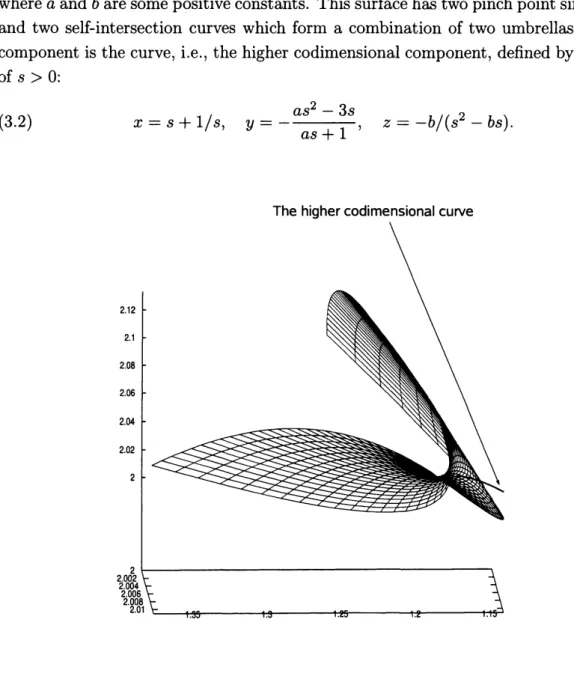
positiveconstants. This surfacehas two pinch pointsingularities

and two self-intersection curves which form a combination of two umbrellas. Another

component is the curve, i.e., the higher codimensional component, definedby equations

of $s>0$:

(3.2) $x=s+1/s, y=- \frac{as^{2}-3s}{as+1}, z=-b/(s^{2}-bs)$_.

Figure 9. $A$ generic slice of the “non-zero $\alpha$

”

$LN$ surface of$T_{3}$ in a transversally

NAOFUMI HONDA AND TAKAHIRO KAWAI

Among other things, the existence of a higher codimensional component of the $LN$

surface that corresponds to the configuration described in Fig. 10 was what we had not

anticipated before the actual computation.

Figure 10. The configuration of vectors $v_{j}’ s.$

Note that the vertex $V_{3}$ may move freely from $V_{2}$ to $V_{4}$ in the configuration of Fig. 10

even if $(p, k)$ is fixed. This flexibility of _{the configuration is tied up with the higher}

codimensionality of the component in question.

We believe that several intriguing features of $L^{+}(T_{3})$ should be tied up with the

existence of non-external vertex $V_{3}$. Here, and in what follows, we say that a vertex is

non-external ifno_{external line is incident upon the vertex. It is probably worth noting}

the following fact.

Let us consider the followinggraph $\overline{T_{3}}$:

Figure 11. The Feynman graph $\overline{T_{3}}.$ Then, for any point $p$ in $L^{\oplus}(\overline{T_{3}})(\subset L^{+}(T_{3}))$,

we

find

(3.3) $p_{6}^{2}=m^{2}$;

otherwise stated, although the external line $p_{6}$ is originally assumed not necessarily

to be on-shell, the current configuration forces it to be on-shell. We note that

we

encountered asimilarsituationinSection 2; at some particular pointsof$L^{\oplus}(G_{1}),$$p_{6}$ lies

on mass-shell. But this time at all points in$L^{\oplus}(\overline{T_{3}}),$

$p_{6}$ obeys themass-shell constraint.

The confirmation of (3.3) is straightforward. First

we

note that the energy-momentum

conservation at $V_{3}$ (i.e., the first equation of (1.6) with $j=3$)

(3.4) $k_{5}=k_{6}=k_{2}=k_{3},$

because $v=2$ and $\alpha_{\ell}\geq 0(\ell=2,3,5,6)$

.

Then it follows from the third equation of

(1.6) that

(3.5) $\alpha_{4}k_{4}=\alpha_{3}k_{3}+\alpha_{5}k_{5}=(\alpha_{3}+\alpha_{5})k_{3},$

and hence

(3.6) $k_{4}=k_{3}.$

Similarly the third equation of (1.6) applied to the triangle formed by $V_{3},$ $V_{4}$ and $V_{5}$

entails

(3.7) $\alpha_{6}k_{6}=\alpha_{5}k_{5}+\alpha_{7}k_{7}.$

Hence (3.4) guarantees

(3.8) $k_{7}=k_{5}=k_{3}.$

Thus the energy-momentum conservation at $V_{4}$ implies

(3.9) $p_{6}=k_{3},$

proving (3.3). In passing, we note that in the

course

of the above reasoning we have

also confirmed

(3.10) $p_{4}+p_{5}=2p_{6}.$

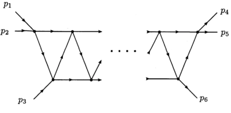
The degeneration of this sort is a universal one, and we can confirm that at a point

$p$ in $L^{\oplus}(T_{n})(n\geq 4)$ where $T_{n}$ is the truss-bridge graph given in Fig. 12 below, all the

internal lines become parallel, and hence we find (in the labeling of external

energy-momentum vectors as in Fig. 12)

(3.11) $p_{4}+p_{5}=2p_{6},$ $p_{6}^{2}=m^{2}$ if$n$ is odd,

and

NAOFUMI HONDA AND TAKAHIRO KAWAI

Figure 12. The truss-bridge graph $T_{n}$ consisting of $n$-trusses.

We also note

(3.13) $p_{1}+p_{2}=2p_{3}, p_{3}^{2}=m^{2}$

holds. Hence, by setting

(3.14) $N=N_{+}\cup N_{-},$ where (3.15) $N_{+}= \bigcup_{p_{3}^{2}=m^{2}}\{(p_{1},p_{2},p_{3});p_{1}+p_{2}=2p_{3}\}$ and (3.16) $N_{-}= \bigcup_{p_{6}^{2}=m^{2}}\{(p_{4},p_{5},p_{6});p_{4}+p_{5}=2p_{6}\},$ we find (3.17) $L^{\oplus}(T_{n})\subset N (n\geq 4)$

with some change of labeling of $(p_{4}, p_{5},p_{6})$ ifnecessary. Thus the micr$0$-analytic

struc-ture of the $S$-matrixnear $N$ should be formidably difficult to study, but we believe the

analysis of individual Feynman integrals $F_{T_{n}}(p)$ should be within reach ofus.

\S 4. Concluding remarks and future problems

Having in mind the study of micro-analytic structure of the $S$-matrix near the

3-particle threshold, we have made a detailed study of the $LN$ surfaces associated with

an ice-cream cone graph and a truss-bridge graph $T_{n}$ with $n=3$ near the 3-particle

threshold. Thanks to the power of recent computers

our

results

are

precise enough to stimulate the interest of mathematicians in the geometry of $LN$ surfaces

near

the

3-particle threshold. Among other things we note that a central role is played by the

set $N$ given by (3.14) (or $N$-for the configuration of Fig. 4). Although the singularity

structure ofthe $S$-matrix near $N$ should be too complicatedto analyze, we believe the

studyof the holonomic structure of individual Feynman integrals near $N$ is an

interest-ing problem inmicrolocal analysis. Another interesting feature ofour results is that the

existence of non-extemal vertices in a Feynman graph normally gives strong constraint

on the shape of the associated $\ovalbox{\tt\small REJECT}\gamma$ variety. (See [4] and [5] for some related topics.)

The studyof the holonomic structure ofaFeynman integral associated with a Feynman

graph containing non-external vertices is an important and challenging problem in mi-crolocal analysis. One natural way to approach this problem is to introduce fictitiously

an external vector $p_{j}$ at anon-external vertex $V_{j}$ and then set it to be $0$

.

As one

imme-diately realizes, this procedure normally leads to the restriction ofa holonomic system

to a submanifold which contains characteristic points. We believe concrete studies of

Feynman integrals of this sort should contribute much to the progress of the theory of

holonomic systems.

References

[1] Eden, R. J., Landshoff, P. V., Olive, D. I. and Polkinghome, J. C., The Analytic $S$-matrix,

Cambridge Univ. Press, 1966.

[2] Sato, M., Recent development in hyperfunction theory and its applications to physics, Intemational SymposiumonMathematical Problems in TheoreticalPhysics (H. Araki, ed.),

Lect. Notes in Phys. 39, Springer, 1975, pp. 13-29.

[3] Kashiwara, M. andKawai, T., Feynmanintegralsandpseudo-differential equations, S\^ugaku

29, 1977, pp. 254-268 (in Japanese).

[4] Kawai, T. and Stapp, H. P., Microlocal study of $S$-matrix singularity structure,

Intema-tional Symposium on Mathematical Problems in TheoreticalPhysics (H. Araki, ed.), Lect.

Notes in Phys. 39, Springer, 1975, pp. 38-48.

[5] –, On the regular holonomic character of the $S$-matrix and microlocal analysis of