Short-wavelength analysis of magnetorotational instability of resistive MHD flows (Mathematical Analysis of Viscous Incompressible Fluid)

全文

(1)78. 数理解析研究所講究録第2058巻 2017年 78-89. Short‐wavelength analysis of magnetorotational instability of resistive MHD flows. Yasuhide Fukumoto Institute of Mathematics for. Industry, Kyushu University Rong Zou College of Mathematics, Physics and Information Engineering, Zhejiang Normal University Oleg Kirillov Steklov Mathematical Institute, Russian Academy of Sciences, Moscow, Russia. Abstract. stability analysis is made of axisymmetric rotating flows of a per‐ fectly conducting fluid and resistive flows with viscosity, subjected to exter‐ nal azimuthal magnetic field B_{ $\theta$} to non‐axisymmetric as well as axisymmet‐ \mathrm{r}\mathrm{i}\mathrm{c} perturbations. For perfectly conducting fluid (ideal MHD), we use the Hain‐Lüst equation, capable of dealing with perturbations over a wide range of the axial wavenumber k to take short wavelength approximation. When the magnetic field is sufficiently weak, the maximum growth rate is given by the Oort \mathrm{A} ‐value |Ro| where $\Omega$(r) is the angular velocity of the rotating flow as a function only of r the distance from the axis of symmetry, and the prime designates the derivative in r As the magnetic field is increased, the keplerian flow becomes unstable to waves of short axial wavelength when Rb=r^{2}(B_{ $\theta$}/r)'/(2B_{ $\theta$})>-3/4 with growth rate proportional to |B_{ $\theta$}| We also incorporate the effect of the viscosity and the electric resistivity and ap‐ ply the WKB method in the same way as we do to the perfectly conducting fluid. In the inductionless limit,i.e. when the magnetic diffusivity is much larger than the viscosity, Keplerian‐rotation flow of arbitrary distributions of the magnetic field, including the Liu limit, becomes unstable. Local. ,. ,. .. ..

(2) 79. 1. Introduction. Since. rediscovery of Velikhov and Chandrasekhars result [1, 2] by Balbus and Hawley [3]\prime the magnetorotational instability (MRI) has attracted great attention as a plausible mechanism for triggering turbulence in the flow of an accretion disk, for promoting outward transport of angular momentum, while the matter accretes the center. There is a well known Rayleighs criterion for stability of a rotating flow of circular streamlines [4]. Given the angular velocity $\Omega$(r) as a function only of the distance r from the rotation axis, define the local Rossby number by Ro= \displayte\frac{1}2 dlog $\Omega$/\mathrm{d}\log r=r$\Omega$'/(2 $\Omega$)[5 6 ] Here the prime designates the derivative with respect to r In terms of the epicyclic frequency $\kappa$^{2}=($\Omega$^{2}r^{4})'/r^{3} it is expressed as Ro=\mathrm{K}^{2}/(4$\Omega$^{2})-1 If $\kappa$^{2}\geq 0 or Ro\geq-1 everywhere, such a rotating flow is linearly stable against axisymmetric disturbances [4, 6]. For an accretion disk, the angular velocity could satisfy the Keplerian law: $\Omega$(r)^{2}r=-\nabla $\Phi$ ; $\Phi$=1/r, for which Ro=-3/4 Rayleighs criterion may suggest that Keplerian rotation $\Omega$\propto r^{-3/2} is hydrodynamically stable. The magnetic field parallel to the rotation axis drastically alters the stability characteristics. If the axial magnetic field is applied, however weak it is, a rotat‐ ing flow suffers from instability if Ro<0[1 2 ] implying that an accretion disk with Keplerian flow is unstable. We refer this instability to the standard mag‐ netorotational instability (SMRI). The maximum growth rate at a local portion was found to be 3| $\Omega$|/4 for a Keplerian rotation [7]. Foì} a general rotating flow of differential rotation $\Omega$(r) satisfying Ro<0 the most unstable local instability mode of the SMRI is the axisymmetric one, with the maximum growth rate being v_{A}/ $\Omega$=\displaystyle \frac{1}{2}|\mathrm{d}\log $\Omega$/\mathrm{d}\log r| the Oort A ‐value [7]. A distinguishing feature is that this growth rate is independent of the applied field strength. When the magnetic field is frozen into the fluid, the differential rotation of the flow generates the azimuthal component of the magnetic field once the magnetic field acquires the radial component which is possibly created by perturbing the axial field [8, 9]. Hence, it is worthwhile to look into the stability of a rotating flow applied by the azimuthal magnetic field and by a combination of the azimuthal and the axial magnetic field. The instability of the former case is called the azimuthal MRI or the AMRI, and the latter is called the helical MRI or the HMRI [5]. The HMRI has been extensively studied for a fluid of very low conductivity, called the inductionless limit [10, 5], because this is relevant to the experimental setting of using a liquid metal of very low conductivity [11]. Recently, an elaborate analysis has also been made for the AMRI in the regime of very low conductivity [12, 13]. For the perfectly conducting case, the AMRI and the HMRI to three‐dimensional ,. ,. .. .. ,. .. .. ,. ,. ,. ,.

(3) 80. disturbances of short. wavelength were both. examined. numerically by Balbus and Hawley [8]. They showed occurrence of the instability by conducting numer‐ ical computation of linearized equations made simplified by leaving out, by a physical intuition, terms which appeared to be less important when the spatial variation of the basic magnetic field is slow. But they did not give the values of the growth rate or the parameter region for instability. Define magnetic Rossby number Rb=r^{2}(B_{ $\theta$}/r)'/(2B_{ $\theta$}) [14] Ogilvie and Pringle [15]addressed three‐ dimensional AMRI by not only the short‐wavelength but also the global analyses. By the former analysis, they showed that, in the limit of the axial wavenumber k\rightarrow\infty the maximum growth rate approaches the Oort \mathrm{A}‐value in the weak‐field .regime, while that, in the same limit, the instability occurs for magnetic Rossby number Rb>-3/4 in the strong‐field regime. We point out that the traditional treatment of the short‐wave stability analysis is liable to miss some terms if a WKB‐form of the solution is substituted at an early stage. For a circular symmet‐ ric flow, the equation for the radial displacement field is known as the Hain‐Lüst equation [16, 17]. We resort to the Hain‐Lüst equation, as augmented with the terms of the basic flow, in its full form, for the AMRI to non‐axisymmetric as well as axisymmetric disturbances. With this equation at hand, we are capable of exploring the local instability over a wide range of k And the same idea is used when the viscosity and electric resistivity are included. .. ,. .. 2. Equations. We consider. and. short‐wavelength approximation. symmetric flow of an incompressible inviscid fluid with infinite electric conductivity, subjected to a steady extemal magnetic field, and the linear stability of a localized disturbance along one of the streamlines. We assume that the radial wavelength is mùch small compared with the radius r of the streamline, being a sort of the WKB approximatiotì. We introduce global cylindrical coordinates (r, $\theta$,z) with the z ‐axis lying on the symmetric axis. The basic state is a rotating flow in equilibrium, with the angular velocity $\Omega$(r) subject to a magnetic field having the azimuthal and the axial components B_{ $\theta$}(r)=r $\mu$(r) and B_{z}. a. circular. ,. U=r $\Omega$(r)e_{ $\theta$}, B=r $\mu$(r)e_{ $\theta$}+B_{z}e_{z}. (1). ,. where e_{ $\theta$} and e_{z} are the unit vectors in the azimuthal and the axial directions, respectively. We mainly focus on the azimuthal field. Denote. \tilde{ $\lambda$}= $\lambda$+im $\Omega$. pressure to be ũ,. .. Assume disturbance of. \tilde{B} and \tilde{p} and. a new. variable. velocity, magnetic. $\chi$=-ru_{r}/\tilde{ $\lambda$}. field and. associated with the.

(4) 81. radial. Lagrangian displacement [16].. We have the Hain‐Lüst. \displayst le\frac{\mathrm{d} \mathrm{d}r(f\rac{\mathrm{d}$\chi$}{\mathrm{d}r)=g$\chi$ where, by. use. of the definition. equation [17], (2). ,. h^{2}=m^{2}/l^{2}+k^{2},. f=\displaystyle\frac{1}{h^{2_{$\gam a$} (\tilde{$\lambda$}^{2}+\frac{F^{2}{p$\mu$_{0}) g=\displaystyle\frac{\mathrm{d}{\mathrm{d}r[\frac{2im}{h^{2}r^{2}($\Omega$\tilde{$\lambda$}-\frac{i$\mu$F}{p$\mu$_{0})]+\frac{1}{r(\tilde{$\lambda$}^{2}+\frac{F^{2}{p$\mu$_{0}) ,. (3) .. +\displaystle\frac{\mathrm{d}$\Omega$^{2}\mathrm{d}r-\fac{1}p$\mu$_{0}\frac{\mathrm{d}$\mu$^{2}\mathrm{d}r+\frac{4k^2}($\Omega$\tilde{$\lambda$}- \mu$iF/(\sqrt{}$\mu$_{0})^{2}h^{2}r(\tilde{$\lambda$}^{2+F^{2}/(p$\mu$_{0}) ,. Here thé. magnetic permeability $\mu$_{0} the density p are assumed to be constant, and F=m $\mu$+B_{z}k We seek the solution of (2) in the WKB approximation. For this purpose, we substitute into (2) the form $\chi$(r)=p(r)\displaystyle \exp[i\int q(r)\mathrm{d}r] with the constraint that the radial wavelength 2 $\pi$/q is assumed to be much shorter than the characteristic length L a measure for radial inhomogeneity, namely, qL\gg 1.. Neglecting the second‐order terms in qL\gg 1 the dispersion relation is gained from (2) as q^{2}=-g/f producing .. ,. ,. ,. (h^{2}+q^{2})(\displaystyle\tilde{$\lambda$}^{2}+\frac{F^{2}{\sqrt{}$\mu$_{0})^{2}+4k^{2}($\Omega$\tilde{$\lambda$}-\frac{i$\mu$F}{p$\mu$_{0})^{2}. +4h^{2}[\displayst le\frac{imr}{2\frac{\mathrm{d} \mathrm{d}r(\frac{$\Omega$\tilde{$\lambda$}-\frac{i$\mu$F}{p$\mu$_{0} {h^2}r^{2})+$\Omega$^{2}Ro-.\frac{$\mu$^{2}{\sqrt{}$\mu$_{0}Rb]. \times. (\displayst le\tilde{$\lambda$}^{2}+\frac{F^2}{p$\mu$_{0}). =0.. (4). Including kinematic viscosity v and electric resistivity $\eta$ repeating the pre‐ procedure and applying the short‐wavelength approximation, we obtain the following algebraic dispersion equation ,. vious. (h^{2}+q^{2})\displaystyle\tilde{$\lambda$}_{$\eta$}^{2}$\Lambda$^{2}+4k^{2}($\Omega$\tilde{$\lambda$}_{$\gam a$}-\frac{iF$\mu$}{p$\mu$_{0}) [$\Omega$Ro(c\displaystyle\mathrm{o}_{$\eta$}- \omega$_{\mathrm{v})+($\Omega$\tilde{$\lambda$}_{$\eta$}-\frac{iF$\mu$}{p$\mu$_{0})] \times. +4 $\Lambda$ h^{2}\tilde{ $\lambda$},. [($\Omega$^{2}Ro-\displaystle\frac{$\mu$^{2} \sqrt{}$\mu$_{0}Rb)+\frac{imr}{2\frac{\mathrm{d} \mathrm{d}r(\frac{$\Omega$\tilde{$\lambda$}_{$\eta$}-\frac{i$\mu$F}{p$\mu$_{0} {h^2}r^{2}\mathrm{I}]. =0 ,. $\Lambda$=\tilde{ $\lambda$}_{v}+F^{2}/\tilde{ $\lambda$}_{r}r \tilde{ $\lambda$}_{v}= $\lambda$+im $\Omega$+$\omega$_{v}, \tilde{ $\lambda$}_{ $\eta$}= $\lambda$+im $\Omega$+$\omega$_{ $\eta$} $\omega$_{\mathrm{v} =|k|^{2}v and $\omega$_{ $\eta$}=|k|^{2} $\eta$.. where. ,. (5). ,. with. use. of.

(5) 82. For. purpose of stability analysis, it is expedient to define two kinds of Alfvén frequency $\omega$_{A} and $\omega$_{A $\theta$} along with their ratio $\beta$(r) representing the helical our. ,. geometry of the. In. addition,. magnetic field,. q)A=\displaystyle\frac{kB_{z}{\sqrt{p$\mu$_{0}' $\omega$_{A$\theta$}=\frac{$\mu$}{\sqrt{p$\mu$_{0} , $\beta$=\frac{$\omega$_{A$\theta$}{$\omega$_{A}. we. .. (6). introduce three dimensionless parameters, namely, the magnetic Reynolds number Re and the Hartmann number Ha. Prandtl number Pm, the. Pm=\displaystyle\frac{$\omega$_{v}{$\omega$_{$\eta$},Re=\frac{$\Omega$}{$\omega$_{\mathrm{v} ,Ha=\frac{$\omega$_{A}{\sqrt{$\omega$_{v}$\omega$_{$\eta$} The. in. dispersion relation for non‐dimensional variables, (5) being expanded out, leads to. .. (7). with the derivative terms. ($\Lambda$_{1}$\Lambda$_{2}+\displaystyle\overline{Ha}^{2})^{2}+4\frac{h^{2}($\Lambda$_{1}$\Lambda$_{2}+\overline{Ha}^{2}) {h^{2}+q^{2} (Re^{2}PmRo-$\beta$^{2}Ha^{2}Rb) +\displaystyle \frac{4im($\Lambda$_{1}$\Lambda$_{2}+\tilde{Ha}^{2}) {r^{2}(h^{2}+q^{2}) [ReRo\sqrt{Pm}($\Lambda$_{2}+imRe\sqrt{Pm})-i(2m\sqrt{}+1) $\beta$ Ha^{2}Rb. +(i\displaystyle \overline{Ha} $\beta$ Ha-Re\sqrt{Pm}$\Lambda$_{2})\frac{k^{2} {h^{2} ]+4$\alpha$^{2}[(Re$\Lambda$_{2}\sqrt{Pm}-i\overline{Ha} $\beta$ Ha) \times(Re$\Lambda$_{2}\sqrt{Pm}-i\overline{Ha} $\beta$ Ha+RoRe(1-Pm))] =0 ,. (8). where. $\Lambda$_{1}. =. \displayte\frc{$lambd}{$\Omega}. Re. \sqrt{Pm}+imRe\sqrt{Pm}+\sqrt{Pm},. $\Lambda$_{2} = \displaystyle \frac{ $\lambda$}{ $\Omega$}Re\sqrt{Pm}+imRe\sqrt{Pm}+\frac{1}{\sqrt{Pm} ,. \overline{Ha} = Ha(1+m $\beta$) $\alpha$^{2} =. k^{2}. \overline{h^{2}+q^{2} .. ,. (9).

(6) 83. 3. Axisymmetric perturbations for perfectly conduct‐ ing fluid. For the. SMRI, the dispersion relation (4) simplifies, when m=0. \displayst le\frac{$\lambda$^{2} $\Omega$^{2}+Ro(\frac{$\lambda$^{2} $\Omega$^{2}+\frac{$\omega$_{A}^{2} $\Omega$^{2})+\frac{1}4$\alpha$^{2}(\frac{$\lambda$^{2} $\Omega$^{2}+\frac{$\omega$_{\mathcal{A}^{2} $\Omega$^{2})^{2}=0 where. $\alpha$=k/\sqrt{q^{2}+k^{2}}. boundary. .. We read off from. (10) limited. to. to. ,. (10). ,. $\lambda$=0 the stability. as. Ro_{c}=-\displaystyle\frac{$\omega$_{A}^{2} {4$\alpha$^{2}$\Omega$^{2} (<0). ,. or. \displayst le\frac{$\omega$_{A}{$\Omega$}=0. (11). .. For the azimuthal MRI. (AMRI), for which the magnetic field has an azimuthal component B=r $\mu$(r)e_{ $\theta$} only. For the axisymmetric case (m=0) the growth rate calculated from (4) is ,. $\lambda$=\pm 2 $\Omega \alpha$\sqrt{-1-Ro+Rb$\omega$_{A $\theta$}^{2}/$\Omega$^{2} , $\lambda$=0 where. $\omega$_{A $\theta$}= $\mu$/\sqrt{\sqrt{}$\mu$_{0}. ,. and $\lambda$=0 is. a. double root. The. (12). ,. instability region is Ro<. $\omega$_{A $\theta$}^{2}/$\Omega$^{2}-1 i.e., the critical Rossby number Ro_{c}=Rb$\omega$_{A $\theta$}^{2}/$\Omega$^{2}-1 which recovers Michaels criterion [19] (See also refs [2, 20 Recently, this criterion is extended to include the viscosity and the electric resistivity [13].. Rb. 4. ,. ,. Non‐axisymmetric perturbations:. weak. magnetic. field magnetic field B=r $\mu$(r)e_{ $\theta$} We start with the case of a very weak magnetic field. By trial and error of numerical calculation, it is probable that the maximum growth rate is attained in the limit of k\rightarrow\infty The dispersion relation (4) reduces, in the limit of k^{2}+q^{2}\rightarrow\infty and $\omega$_{A}\rightarrow 0 to Hereafter. we. restrict to azimuthal. .. .. ,. 4(\displaystyle\tilde{$\lambda$}$\Omega$-im$\omega$_{A$\theta$}^{2})^{2}+\frac{1}{$\alpha$^{2} (\tilde{$\lambda$}^{2}+m^{2}0\mathrm{J}_{A$\theta$}^{2})^{2}. +(\tilde{ $\lambda$}^{2}+m^{2}$\omega$_{A $\theta$}^{2})(4$\Omega$^{2}Ro-4Rb$\omega$_{A $\theta$}^{2})=0. .. (13). Equation (13), which is valid for a strong magnetic field as well, was derived by Ogilvie and Pringle [15], and coincides with the dispersion relation of the work [13] if the viscous and resistive terms are dropped off..

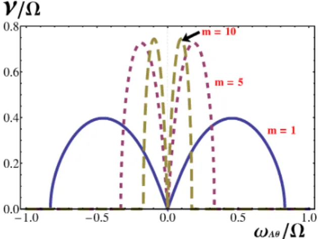
(7) 84. Figure 1: The growth rate, in the limit k\rightarrow\infty with fixing $\alpha$= 1 of the non‐ axisymmetric AMRI versus $\omega$_{A $\theta$}/ $\Omega$ in the range of small values, for different azimuthal wavenumbers m=1 (solid line), 5 (dashed line) and 10 (long dashed line) for Ro=-3/4 a Keplerian rotation. The magnetic Rossby number is Rb= ,. ,. ,. -1.. growth rate increases with |m|. Interestingly, growth approaches, as |m| is increased, the same value as that of the SMRI as found by Ogilvie and Pringle [15]. Fig. 1 displays the growth rate $\sigma$={\rm Re}[$\lambda$_{3,4}] as functions of the Alfvén frequency $\omega$_{A $\theta$} with azimuthal Given. a. small value of. |$\omega$_{A $\theta$}/ $\Omega$|. the maximum. wavenumbers. m=. 1. ,. ,. the maximum. rate. 5 and 10 for. Ro=-3/4. is. and Rb=-1. Since the system corresponds the growing .. Hamiltonian, to each damping perturbation ( $\sigma$<0) perturbation ( $\sigma$>0) and therefore we display only the solution with positive real part $\sigma$ The change of the sign of Rb, namely, the choice of Rb=1 does not change much the growth rate. We observe from Fig. 1 that, as m increases, the .. ,. growth rate approaches 3| $\Omega$|/4 though the width of the instability band m Indeed, by taking $\omega$_{A $\theta$}/ $\Omega$ m$\omega$_{A $\theta$}^{2}=0 and Rb$\omega$_{\mathrm{A} $\theta$}^{2}=0 in (13) as a limit of small values of |$\omega$_{\mathcal{A} $\theta$}/ $\Omega$| with maintaining |m$\omega$_{A $\theta$}/ $\Omega$| finite, we can show that the maximum growth rate happens to coincides with the Oort \mathrm{A}‐value. maximum in. ,. is narrowed with. $\sigma$_{\mathrm{A} /| $\Omega$|=|Ro|.. ..

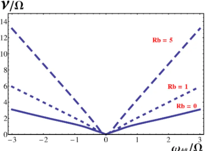
(8) 85. 5. Non‐axisymmetric perturbations: strong. external. field 5.1. Strong fields. Here. and ideal AMRI. the maximum value is taken at for. |$\omega$_{A $\theta$}/ $\Omega$|\sim 1 In the limit of k\rightarrow\infty, | $\alpha$|=1 and at m=0 for Rb\geq 3/4 but at |m|=1. consider ideal MHD with the. we. -3/4<Rb<3/4. ,. case. of. .. ,. ,. with the maximum values. \displayte\frac{$sigma_{\ x}$\Omega$}\proxleft\{bginary}{l 2\sqrt{Rb}|$\omega_{A$\thea}/$\Omega$|\ (Rbgeq3/4)\ sqrt{2Rb-1+\sqrt{1+Rb^2}|$\omega_{A$\thea}/$\Omega$|\ (-3/4<Rb ). \end{ary}\ight.. This value decreases to. Fig.. zero as. 2 shows the. Rb decreases to. rate, for. -3/4.. 1 in the limit of k\rightarrow\infty. growth range of the Alfven frequency $\omega$_{A $\theta$}/ $\Omega$ and for typical values the range of Rb>-3/4 The flow is Keplerian (Ro<0) m=. .. Strong fields. 5.2 We. are. (14). of Rb. ,. over a. wide. (=0 1, 5 ) ,. in. .. and inductionless AMRI. concerned with the inductionless limit and. of Pm\rightarrow 0 and Ha\rightarrow 0 in. (8),. we. rotating. flow.. Taking. the limit. get. \displaystyle \hat{ $\lambda$}^{2}+\frac{4\hat{ $\lambda$} {(h^{2}+q^{2})r^{2} \{Ha_{ $\theta$}^{2}(2m^{2}Rb-h^{2}r^{2}Rb-\frac{k^{2}m^{2} {h^{2} )+imRe(Ro-\frac{k^{2} {h^{2} )\} +4$\alpha$^{2}(Re- imHa_{ $\theta$}^{2})(Re-imHa_{ $\theta$}^{2}+ReRo)=0. where and. \hat{ $\lambda$}=1+Ha_{ $\theta$}^{2}m^{2}+ $\lambda$ Re/ $\Omega$+imRe and. Ha_{ $\theta$}=$\omega$_{A $\theta$}/\sqrt{$\omega$_{\mathrm{v} $\omega$_{ $\eta$}. (15), the eigenvalues. \displayte\frac{$lmbda_{1}$\Omega} \displayte\frac{$lmbda_{2}$\Omega}. =. =. .. Taking. we. (15). ,. recall. $\alpha$^{2}=k^{2}/(k^{2}+q^{2}+m^{2}/r^{2}). the limit of k\rightarrow 0 thus $\alpha$\rightarrow 0 and ,. h\rightarrow m/r. ,. of. become. -im-(1+Ha_{ $\theta$}^{2}m^{2})\displaystyle \frac{1}{Re}. ,. -im(1+\displaystyle \frac{4Ro}{m^{2}+q^{2}r^{2} )-[1+Ha_{ $\theta$}^{2}m^{2}(1+\frac{4Rb}{m^{2}+q^{2}r^{2} )]\frac{1}{Re}. .. (16).

(9) 86. Figure 2: The growth rate, for m=1 and k\rightarrow\infty with fixing $\alpha$=1 of the non‐ axisymmetric AMRI over a wide range of $\omega$_{A $\theta$}/ $\Omega$ for negative Ro=-3/4 and dif‐ ferent non‐negative magnetic Rossby numbers Rb: Rb=0 (solid line), 1 (dashed line) and 5 (long dashed line). ,. We. immediately. find the. instability region. Rb<-\displaystyle \frac{1}{4}(m^{2}+q^{2}r^{2}). and. as. Ha_{$\theta$}^{2}>\displaystyle\frac{1}{m^{2}(\frac{4|Rb|}{m^{2}+q^{2}r^{2}-1)}. We consider the mode of k\rightarrow\infty for which the ,. \displayte\frac{$\lmbda$_{1,2}$\Omega$}. =. eigenvalues. .. (17). are. \displaystyle \frac{2$\alpha$^{2}Ha_{ $\theta$}^{2}Rb-1-m^{2}Ha_{ $\theta$}^{2} {Re}-im \displaystyle \pm 2 $\alpha$\{\frac{Ha_{ $\theta$}^{4} {Re^{2} (m^{2}+$\alpha$^{2}Rb^{2})-(1+Ro)+im\frac{Ha_{ $\theta$}^{2} {Re}(2+Ro)\}^{\frac{1}{2}. (18). instability occurs when Ro<-1 with growthrate $\lambda$_{R}/ $\Omega$\approx 2 $\alpha$\sqrt{-(1+Ro)}. pertains to the classical Rayleigh instability since no magnetic field is required. When Ro>-1 the instability criterion becomes The. This mode. ,. 2$\alpha$^{2}Rb-m^{2}+\displaystyle \frac{| $\alpha$ m|(2+Ro)}{\sqrt{1+Ro} >0, and. Ha_{ $\theta$}^{2}>\displaystyle \frac{\sqrt{1+Ro} {(2$\alpha$^{2}Rb-m^{2})\sqrt{1+Ro}+|\mathrm{a}m|(2+Ro)}. .. (19).

(10) 87. Rb<-1/4 is necessary for the instability of \mathrm{m}=1 mode as shown by (17), while in the short‐wave limit of k=\infty, Rb> −25/32 is necessary for the instability that is attained at m/ $\alpha$=\pm 5/4 Because the, later In the. long‐wave. limit of k\rightarrow 0,. .. overlaps with the former one, we conclude that the instability exists for arbi‐ trary magnetic Rossby number. Either the mode of k\rightarrow 0 or k\rightarrow\infty dominate in large range of Rb, and the maximum growth rate is attained at finite value of k in a narrow range of Rb as illustrated by FIG. 3. FIG. 3 draws the growth rate against the magnetic Rossby number Rb for Re=10^{4}, Ha_{ $\theta$}=100, m=1 and Ro=-3/4. We observe the crossover of the k=0, q=0 mode to the k=\infty mode. The range of small value of Rb is dominated by the k=0 mode and the one of large values of Rb is dominated by the k\rightarrow\infty mode. one. magnetic Rossby number Rb for Re=10^{4}, Ha_{ $\theta$}= 100, m=1 and Ro=-3/4 solid line is k=0, q=0 mode, Dotted one is the k=\infty mode and dashed line stands for the maximum growth rate, whose left part coincide with the k=0 mode and the right part coincides with the k=\infty, $\alpha$=1. Figure. 3: the. growth. rate to. .. ,. mode.. References [1] E. Velikhov, JETP (USSR) 3ó, 1398 (1959). [2] S. Chandrasekhar, Proc. Natl. Acad. Sci. 4ó, 253 (1960). [3] A. Balbus, and J. $\Gamma$ Hawley, Astrophys. J. 37ó, 214 (1991). ..

(11) 88. [4] S. Chandrasekhar, Hydrodynamic and Hydromagnetic Stability (Clarendon Press, Oxford, 1961).. [5] O. N. Kirillov, and $\Gamma$ Stefani, Astrophys. J. 712, 52 (2010). .. [6] O. N. Kirillov, and $\Gamma$ Stefani, Acta Appl. Math. 120, 177 (2012). .. [7] A. Balbus, and J. $\Gamma$ Hawley, Astrophys.. J.. 392, 662 (1992).. [8] A. Balbus, and J.. J.. 400, 610 (1992).. .. $\Gamma$. .. Hawley, Astrophys.. [9] S. J. Desch, Astrophys. J. ó08, 509 (2004). [10] R. Hollerbach, and G. Rüdiger, Phys. Rev. Lett. 95, 124501 (2005).. [11] F. Stefani, Th. Gundrum, G. Gerbeth, G. Rüdiger, M. Schultz, J. Szklarski, and R. Hollerbach, Phys. Rev. Lett. 97, 184502 (2006). [12] G. Rüdiger, M. Gellert, M. Schultz, R. Hollerbach, and F. Stefani, Mon. Not. R. Astron. Soc. 438, 271 (2014). [13] O. N. Kirillov, $\Gamma$ Stefani, and Y. Fukumoto, Fluid Dyn. Res. 4ó, 031403 (2014). .. [14] O. N. Kirillov, and $\Gamma$ Stefani, Phys. Rev. Lett. 111, 061103 (2013). .. [15] G. I. Ogilvie, and J. E. Pringle, Mon. Not. R. Astron. Soc. 279, 152 (1996). [16] J. P. Goedbloed, and S. Poedts, Principles ofMagnetohydrodynamics (Cam‐ bridge University Press. Cambridge, 2004). [17] J. P. Goedbloed, R. Keppens, and S. Poedts, Advanced Magnetohydrody‐ namics. (Cambridge University Press. Cambridge, 2010).. [18] O. N. Kirillov, and $\Gamma$ Stefani, Phys. Rev. E84, 036304 (2011). .. [19] D. H. Michael, Mathematika 1, 45 (1954). [20] E. KnobIoch, Mon. Not.. R. Astron. Soc.. 255, 25 (1992).. [21] A. B. Mikhailovskii, J. G. Lominadze, R. M. O. Galvao, A. P. Churikov, N. N. Erokhin, A. I. Smolyakov, and V. S. Tsypin, Phys. Plasmas 15, 0521038 (2008)..

(12) 89. [22] R. J. Tayler, Mon. Not. R. Astron. Soc. lól, 365 (1973). [23] P. G. Saffman, Vortex Dynamics (Cambridge University Press. Cambridge, 1992).. [24] Y. Fukumoto, J. Fluid Mech. 493, 287 (2003)..

(13)