Topology and Differentiable Structures of Mapping Space Quotients (Singularity theory of differential maps and its applications)

全文

(1)1. 数理解析研究所講究録第2049巻 2017年 1-21. Topology and Differentiable Structures Mapping Space Quotients. of. Goo ISHIKAWA. Abstract In this survey article we show the basic method how to give topological structures mapping spaces or mapping space quotients and moreover introduce a new method provide differentiable structures on them with illustrative examples.. 1. on. to. Introduction.. To describe. complicated phenomena, we need an infinite number of parameters, since our real has, of course, infinite dimension. However, on the other hand, we are able to under‐ stand fully only finite dimensional objects. Therefore we have to pick up a finite number of parameters, according to each purpose, among an infinite number of parameters. We extract finite dimensional objects from infinite dimensional objects and naturally such parameters enjoy several relations or conditions. Thus we proceed to study finite dimensional manifolds. In this stage, geometrical study plays an important role. Then, in the study of finite dimen‐ sional manifolds, functions on manifolds and mappings between manifolds are investigated. The space of mappings are of infinite dimensional. Then, again we extract finite dimensional objects from infinite dimensional mapping spaces. Thus our understanding is improved, step by step, on various complicated phenomena and the mathematical structures behind them as well. Now we are going to start with finite dimensional manifolds. Let N, M be differentiable manifolds of dimension n, m respectively. In this article we only treat c\infty i.e. infinitely differentiable manifolds and c\infty mappings, otherwise stated. Let C^{\infty}(N, M) denote the set of differentiable mappings from N to M and X be a subset of C^{\infty}(N, $\Lambda$ I) is given on X Then X/\sim denotes the Suppose an equivalence relation quotient space (mapping space quotient). The problem is how to give a topological structure and a differentiable structure on the mapping space quotient X/\sim. world. ,. \sim. .. .. Example 1.1 (The space of knots.) An embedding from the circle S^{1} to the space \mathrm{R}^{3} or its image is called a knot. Let \mathrm{E}\mathrm{m}\mathrm{b}(S^{1}, \mathrm{R}^{3})\subset C^{\infty}(S^{1}, \mathrm{R}^{3}) denote the set consisting of knots (the space of knots). Then the knot theory treats connected components of the space of knots \mathrm{E}\mathrm{m}\mathrm{b}(S^{1}, \mathrm{R}^{3}) Moreover we can define on it various geometric structures (e.g. a symplectic structure, a complex structure and so on. See [8]. See also subsection 6.3 of this article. .. (The diffeomorphism group.). The space \mathrm{D}\mathrm{i}\mathrm{f}\mathrm{f}(N) of diffeomorphisms on N can topological group and an infinite dimensional Lie group. For example the famous theorem stating that the space \mathrm{D}\mathrm{i}\mathrm{f}\mathrm{f}^{+}(S^{2}) of orientation‐preserving diffeomorphisms on the sphere S^{2} is homotopy equivalent to the special orthogonal group SO(3) need the topology on the mapping space \mathrm{D}\mathrm{i}\mathrm{f}\mathrm{f}^{+}(S^{2}). Example. 1.2. be endowed with the structure of. a. ..

(2) 2. Example. (The. 1.3. nian structures. super space of Riemannian structures.. N. Then \mathcal{R}_{N} is. regarded. ). Let \mathcal{R}_{N} be the set of Rieman‐. mapping space. The diffeomorphism group acts on and the orbit \mathcal{R}_{N} \mathrm{D}\mathrm{i}\mathrm{f}\mathrm{f}(N) naturally space or the quotient space \prime R_{N}/\mathrm{D}\mathrm{i}\mathrm{f}\mathrm{f}(N) which is is the of designated by S_{N} space isomorphisms classes of Riemannian structures on N which on. .. as a. ,. is called the super space. See subsection 6.4.. Example 1.4 (The variational method.) Let $\Phi$ $\Phi$(f) be a real valued function on the Then the a differentiable mapping from N variable means mapping space C^{\infty}(N, M) f A mapping f \in C^{\infty}(N, M) is called a critical point of $\Phi$ if, for any one‐parameter to M =. .. .. deformation on. C^{\infty}(N, M). Example. \displaystyle \frac{d}{dt} $\Phi$(f_{t})|_{t=0}=0. f_{\mathrm{t} ,. .. Based. this. on. idea,. later. we. will. give a differentiable structure. See section 5.. .. (Stability. 1.5. and the classification problem of mappings.) On the mapping space product group \mathrm{D}\mathrm{i}\mathrm{f}\mathrm{f}(N) \times \mathrm{D}\mathrm{i}\mathrm{f}\mathrm{f}(M) of diffeomorphism groups naturally acts. Then we call a mapping f\in C^{\infty}(N, M) is stable if the orbit through f forms an open subset of C^{\infty}(N, M) namely if any f' belonging to some neighbourhood of f is transformed to f via the action of \mathrm{D}\mathrm{i}\mathrm{f}\mathrm{f}(N) \times \mathrm{D}\mathrm{i}\mathrm{f}\mathrm{f}(M) The purpose of the differential topology of mapping is to study on the the quotient space \mathcal{M} := C^{\infty}(N, M)/\mathrm{D}\mathrm{i}\mathrm{f}\mathrm{f}(N) \times \mathrm{D}\mathrm{i}\mathrm{f}\mathrm{f}(M) Considering, for each point x_{0} \in N the germ of f \in C^{\infty}(N, M) at x0 we define the equivalence relation \sim_{x_{0}} on the set C^{\infty}(N, M) The quotient space C^{\infty}(N, M)/\sim_{x_{0}} represents the space of germs f : (N, x_{0})\rightarrow M of differentiable mappings. We will give the topology and the differentiable structure on C^{\infty}(N, M)/\sim_{x_{0}} Then the purpose of the singularity theory of mappings is to study on the various (further) quotient spaces of C^{\infty}(N, M)/\sim_{x_{0}}.. C^{\infty}(N, M). the. ,. ,. .. .. ,. ,. .. .. First. recall how to introduce several. we. topologies on mapping spaces in §2 for the case §3 for the case of finite dimensional manifolds. In §4 we treat explain our main theory of differentiable structures on mapping provide several examples and applications of the theory in §6.. of Cartesian spaces, and in the space of map‐germs. We. quotients. space. This paper. §5,. in. and. first. prepared by the author for a lecture at Department of Mathematics, University performed on the autumn‐winter semester of 2004. The manuscript has renewed and arranged on March 2016 by the author. was. Hokkaido been. 2. Topology. We denote Then. by. we. of. spaces between Cartesian spaces. C^{0}(\mathrm{R}^{n}, \mathrm{R}^{m}). define the. generator: For. mapping. a. the set of C^{0} (i.e. continuous) mappings from \mathrm{R}^{n} to \mathrm{R}^{m}. C^{0} ‐topology (or compact open topology) on C^{0}(\mathrm{R}^{n}, \mathrm{R}^{m}) by giving. compact. set K\subset \mathrm{R}^{n} and. an. open set. U\subset \mathrm{R}^{n}\times \mathrm{R}^{m}. we. its. set. W(K, U) :=\{f\in C^{0}(\mathrm{R}^{n}, \mathrm{R}^{m})|j^{0}f(K)\subseteq U\}, where. j^{0}f. W(K, U). :. \mathrm{R}^{n} \rightarrow \mathrm{R}^{n} \times \mathrm{R}^{m} is the. is the set of continuous. is included in the. the. family of. given. subsets of. graph mapping. mapping. such that the. open subset of \mathrm{R}^{n}\times \mathrm{R}^{m}. C^{\infty}(\mathrm{R}^{n},\mathrm{R}^{m}). .. defined. graph. We take. as. j^{0}f(x). by. the the. :. { W(K, U) |K\subset \mathrm{R}^{n}. =. (x, f(x)). .. Then. given compact set the generator of the topology. over. compact, U\subset \mathrm{R}^{n}\times \mathrm{R}^{m}. open}..

(3) 3. Thus, for the C^{0} topology, f\in $\Omega$ there exist compact. a. $\Omega$\subseteq C^{0}(\mathrm{R}^{n}, \mathrm{R}^{m}). subset. K_{1}. set. ,. .. .. .. ,. K_{s}. ,. is. an. open subset if and. in \mathrm{R}^{n} and open subsets. U_{1}. ,. .. .. .. :. only if for any in \mathrm{R}^{n}\times \mathrm{R}^{m},. U_{s}. such that. f\in W(K_{1}, U_{1})\cap W(K_{2}, U_{2})\cap\cdots\cap W(K_{s}, U_{s})\subseteq $\Omega$. Note that if. f\in W(K_{1}, U_{1})\cap W(K_{2}, U_{2}) then there exist a compact set K\subset \mathrm{R}^{n} and an open f\in W(K, U)\subseteq W(K_{1}, U_{1})\cap W(K_{2}, U_{2}) In fact it suffices to set ,. subset U\subseteq \mathrm{R}^{n}\times \mathrm{R}^{m} with. .. K=K_{1}\cup K_{2}, U=($\pi$_{1}^{-1}(K_{1}\cap K_{2})\cap U_{1}\cap U_{2})\cup(U_{1}\backslash $\pi$^{-1}(K_{1}\cap K_{2}))\cup(U_{2}\backslash $\pi$^{-1}(K_{1}\cap K_{2} The topological space C^{0}(\mathrm{R}^{n}, \mathrm{R}^{m}) is a Hausdorff space with respect to C^{0} ‐topology. Namely, for two mappings f, g \in C^{0}(\mathrm{R}^{n}, \mathrm{R}^{m}) f \neq g there exist an open neighbourhood W of f and an open neighbourhood W' of g satisfying W\cap W'=\emptyset. For a compact set L\subset \mathrm{R}^{n} and an open subset V\subseteq \mathrm{R}^{m} we set ,. ,. ,. W'(L, V) :=\{f\in C^{0}(\mathrm{R}^{n}, \mathrm{R}^{m}) |f(L)\subseteq V\}, topology on C^{0}(\mathrm{R}^{n}, \mathrm{R}^{m}) generated by \{W'(L, V) | L\subset \mathrm{R}^{n} compact, V \subseteq topology coincides with the C^{0} ‐topology. Therefore the C^{0} ‐topology can be said as the topology of uniform convergence on compact subsets The product space C^{0}(\mathrm{R}^{n}, \mathrm{R}^{m})\times C^{0}(\mathrm{R}^{n}, \mathrm{R}^{\ell}) is homeomorphic to C^{0}(\mathrm{R}^{n}, \mathrm{R}^{m}\times \mathrm{R}^{\mathrm{e} ) with respect to C^{0} ‐topology. For a positive integer r>0 we denote by C^{r}(\mathrm{R}^{n}, \mathrm{R}^{m}) the set of C^{r} ‐mappings. Then we can induce a topology on the subset C^{r}(\mathrm{R}^{n}, \mathrm{R}^{m}) \subset C^{0}(\mathrm{R}^{n}, \mathrm{R}^{m}) form the C^{0} ‐topology on C^{0}(\mathrm{R}^{n}, \mathrm{R}^{m}) We call it the C^{0} ‐topology on C^{r}(\mathrm{R}^{n}, \mathrm{R}^{m}) and consider the. \mathrm{R}^{m}. open}.. Then this. ,. .. Next Let. f. \mathrm{R}^{n}\rightarrow \mathrm{R}. j\leq n). ,. define the. we :. .. C^{1} ‐topology on C^{1}(\mathrm{R}^{n}, \mathrm{R}^{m}) a C^{1} ‐mapping. Set f= (f_{1}, f2, . . . , f_{m}) where .. \mathrm{R}^{n}\rightarrow \mathrm{R}^{m} be of class. are. the. 1‐jet. ,. C^{1} Consider, by the partial derivatives .. extension of. f:. \displayte\frac{prtialf_{}\partilx_{j}. :. f_{i}=f_{i}(x_{1}, \ldots , x_{n}). :. \mathrm{R}^{n}\rightar ow \mathrm{R}, (1\leq i\leq m, 1\leq. j^{1}f:\mathrm{R}^{n}\rightarrow \mathrm{R}^{n}\times \mathrm{R}^{m}\times \mathrm{R}^{nm}=\mathrm{R}^{n+m+nm} defined For. by a. j^{1}f(x)=(x, f(x), \displaystyle \frac{\partial f_{i} {\partial x_{j} (x). compact. set K\subset \mathrm{R}^{n} and. .. an. The. mapping. open subset. j^{1}f. is. obviously. U\subseteq \mathrm{R}^{n+m+nm}. ,. continuous. set. we. W(K, U) :=\{f\in C^{1}(\mathrm{R}^{n}, \mathrm{R}^{m}) |j^{1}f(K)\underline{\subseteq}U\} The. family. of subsets. { W(K, U) |K\subset \mathrm{R}^{n} compact, U\subseteq \mathrm{R}^{n+nm} open} of. C^{1}(\mathrm{R}^{n}, \mathrm{R}^{m}). C^{1} ‐topology As if the. topology. on. generate. C^{0} ‐topology. is the. a. C^{1}(\mathrm{R}, \mathrm{R}). topology. topology,. is. which is called the. stronger than C^{0} ‐topology.. is the. topology. C^{1} ‐topology. on. C^{1}(\mathrm{R}^{n}, \mathrm{R}^{m}). .. The. of uniform convergence on compact subsets, the C^{1}together with first derivatives on compact. of uniform convergence. subsets.. Similarly we. define the. we. define the. 2‐jet. C^{2} topology. on. C^{2}(\mathrm{R}^{n}, \mathrm{R}^{m}). .. For. a. C^{2} ‐mapping. extension. j^{2}f:\displaystyle \mathrm{R}^{n}\rightar ow \mathrm{R}^{n}\times \mathrm{R}^{m}\times \mathrm{R}^{nm}\times \mathrm{R}\frac{n(n+1)}{2}m. f\in C^{2}(\mathrm{R}^{n}, \mathrm{R}^{m}). ,.

(4) 4. by in. j^{2}f(x)=(x, f(x), \displaystyle \frac{\partial f_{i} {\partial x_{j} (x), \frac{\partial^{2}f_{i} {\partial x\partial x}(x) \displaystyle \mathrm{R}^{n}\times \mathrm{R}^{m}\times \mathrm{R}^{nm}\times \mathrm{R}\frac{n(n+1)}{2}m ,. .. For. a. compact. set K\subset \mathrm{R}^{n} and. open subset U. an. set. we. W(K, U) :=\{f\in C^{2}(\mathrm{R}^{n}, \mathrm{R}^{m})|j^{2}f(K)\subseteq U\}, and consider the. C^{2}(\mathrm{R}^{n}, \mathrm{R}^{m}) Now. we. .. topology generated by the family \{W(K, U)\} consisting C^{2} ‐topology on C^{2}(\mathrm{R}^{n}, \mathrm{R}^{m}). We call it the. introduce the. Taylor polynomials,. of such subsets in. .. jet. space. J^{r}(\mathrm{R}^{n}, \mathrm{R}^{m}). ,. for each r\geq 0. .. Motivating. on. the space of. set. we. J^{r}(\displaystyle \mathrm{R}^{n}, \mathrm{R}^{m})=\mathrm{R}^{n}\times \mathrm{R}^{m}\times \mathrm{R}^{nm}\times \mathrm{R}\frac{n(n+1)}{2}m\times\cdots\times \mathrm{R}^{N}=\mathrm{R}^{M}, where N=. \left(\begin{ar ay}{l} n+r&-1\ r& \end{ar ay}\right)m. ,. and. M=n+m+nm+\displaystyle \frac{n(n+1)}{2}m+\cdots+\left(\begin{ar ay}{l } n+r & -1\ r & \end{ar ay}\right)m=n+\displaystyle \left(\begin{ar ay}{l} n+r\ r \end{ar ay}\right)m. Then, for by. Note. a. C‐mapping f\in C^{r}(\mathrm{R}^{n},\mathrm{R}^{m}). ,. we. define. r. ‐jet. extension. j^{r}f. \mathrm{R}^{n}\rightarrow J^{r}(\mathrm{R}^{n}, \mathrm{R}^{m}). :. j^{r}f(x):= (x, f(x), \displaystyle \frac{\partial f_{i} {\partial x_{j} (x)_{1}\frac{\partial^{2}f_{i} {\partial xk\partial_{\el } (x), \ldots, \frac{\partial^{r}.f_{i} {\partial x_{j_{1} \cdot\cdot\partial x_{j_{r} (x). .. for r\geq s,. that,. J^{r}(\mathrm{R}^{n}, \mathrm{R}^{m})=\{j^{r}f(x_{0}) |x_{0}\in \mathrm{R}^{n}, f\in C^{S}(\mathrm{R}^{n}, \mathrm{R}^{m} Then the C^{r}. \{W(K, U)\}. topology. on. C^{r}(\mathrm{R}^{n}, \mathrm{R}^{m}). is defined. as. the. topology generated by. the. family. of subsets. W(K, U) :=\{f\in C^{r}(\mathrm{R}^{n},\mathrm{R}^{m})|j^{r}f(K)\subseteq U\} of. C^{r}(\mathrm{R}^{n}, \mathrm{R}^{m}). .. Moreover the C^{r}. topology. C^{s}(\mathrm{R}^{n}, \mathrm{R}^{m})\subseteq C^{r}(\mathrm{R}^{n}, \mathrm{R}^{m}) Lastly and. an. we. on. C^{S}(\mathrm{R}^{n}, \mathrm{R}^{m}) (s = r, r+ 1, \ldots, \infty, $\omega$). define the c\infty ‐topology. open subset. is. induced, since. .. U\subseteq J^{r}(\mathrm{R}^{n}, \mathrm{R}^{m}). ,. on. C^{\infty}(\mathrm{R}^{n}, \mathrm{R}^{m}). .. For. \geq 0. r. ,. a. compact. set K\subset \mathrm{R}^{n}. set. W(r, K, U) :=\{f\in C^{\infty}(\mathrm{R}^{n}, \mathrm{R}^{m}) |j^{r}f(K)\subseteq U\}. Then the C^{\infty}. topology. On the space. is defined. \mathcal{O}_{X}^{0} namely. the. as. X=C^{\infty}(\mathrm{R}^{n}, \mathrm{R}^{m}) \subseteq. \mathcal{O}_{X}^{1}. the we. \subseteq. topology generated by \{W(r, K, a sequence of topologies. U. have. \mathcal{O}_{X}^{2}. .. .. .. \subseteq. \displaystyle \bigcup_{r=0^{\mathcal{O}_{X}^{r}=\mathcal{O}_{X}^{\infty} }^{\infty}.. C^{0} ‐topology, the C^{1} ‐topology, the C^{2} ‐topology,. .. ... ,. and the C^{\infty} ‐topology..

(5) 5. Proposition. 2.1 For. $\Phi$ is. a. continuous. ,. the. s=\infty ,. composition of mappings. ,. mapping. an. case. C^{S}(\mathrm{R}^{n}, \mathrm{R}^{m})\times C^{s}(\mathrm{R}^{m}, \mathrm{R}^{\ell})\rightar ow C^{S}(\mathrm{R}^{n}, \mathrm{R}^{f}) $\Phi$(f,g)=g\circ f, on. the C^{r} ‐topology.. $\Phi$(f_{0}, g_{0})=g_{0}\circ f_{0}=h_{0}. We set. Proof:. K\subset \mathrm{R}^{n} and. :. 0\leq r\leq s including the. open. :. \mathrm{R}^{n}\rightar ow \mathrm{R}^{p} Suppose h_{0} \in W(r, K, U) for. a. .. U\subseteq J^{r}(\mathrm{R}^{n}, \mathrm{R}^{\mathrm{e} ) namely, j^{r}h_{0}(K)\subseteq U ,. .. compact. We set. J^{r}(\mathrm{R}^{n}, \mathrm{R}^{m})\times \mathrm{R}^{m}J^{r}(\mathrm{R}^{m}, \mathrm{R}^{\ell}) =\{ (j^{r}f(x0), j^{r}g(y_{0}))\in J^{r}(\mathrm{R}^{n}, \mathrm{R}^{m})\times J^{r}(\mathrm{R}^{m}, \mathrm{R}^{\ell}) f(x_{0})=y_{0}\} and define $\varphi$ : J^{r}(\mathrm{R}^{n}, \mathrm{R}^{m}) \times \mathrm{R}^{m}J^{r}(\mathrm{R}^{m}, \mathrm{R}^{\ell}) \rightarrow J^{r}(\mathrm{R}^{n}, \mathrm{R}^{\ell}) f)(x0). Then $\varphi$ is a continuous mapping which is expressed. A\subset J^{r}(\mathrm{R}^{n}, \mathrm{R}^{m}) B\subset J^{r}(\mathrm{R}^{m}, \mathrm{R}^{\mathrm{e} ) ,. A\times \mathrm{R}^{m}B. ,. by $\varphi$(j^{r}f(x0),j^{r}g(y_{0})) =j^{r}(g\circ by a polynomial. In general, for. set. :=\{j^{r}f(x0), j^{r}g(y_{0})\in A\times B | f(x_{0})=y_{0}\}\subseteq J^{r}(\mathrm{R}^{n},\mathrm{R}^{m})\times \mathrm{R}^{m}J^{r}(\mathrm{R}^{m}, \mathrm{R}^{\ell}). .. Then, from the assumption, we have $\varphi$ ((j^{r}f_{0})(K) \times \mathrm{R}^{m} (j^{r}g_{0})(f_{0}(K))) \subseteq U By Proposition 2.2 below, there exist an open neighbourhood V of (j^{r}f_{0})(K) in J^{r}(\mathrm{R}^{n}, \mathrm{R}^{m}) and an open neighbourhood V' of (j^{r}g_{0})(f_{0}(K)) ) in J^{r}(\mathrm{R}^{m}, \mathrm{R}^{p}) such that V\times \mathrm{R}^{m}V' \subseteq $\varphi$^{-1}U Thus we .. ,. .. have. $\Phi$(W(K, V), W(f_{0}(K), V. Proposition. 2.2. paracompact,. e.g.. \subseteq W(K, U). and. we see. that $\Phi$ is continuous.. \square. ([21][15]) Suppose A, B, P. are Hausdorff spaces, and P locally compact and manifolds. Suppose $\pi$ : A \rightarrow P, $\pi$' : B \rightarrow P are continuous subsets, $\pi$|_{K} : K \rightarrow P, $\pi$'|_{L} : L\rightarrow P proper. Suppose U' is an. A, B, P. are. mappings, K \subseteq A, L \subseteq B open neighbourhood of K\mathrm{X}pL. | $\pi$(a) =$\pi$'(b)\}. A\times B. ,. neighbourhood V' of L. .. =. \{(a, b) \in K \times L | $\pi$(a) = $\pi$(b)\}. Then there exist in B such that. neighbourhood V\mathrm{x}_{P}V'\subseteq U'. an. Remark 2.3 Remark that the C^{r} ‐topology number of subsets. In. open. (r=0,1,2, \ldots, \infty). V. is. in A. of. \times pB. \{(a, b). =. K in A and. generated by. a. an. \in. open. countable. fact,. \{W(r,\overline{U_{1/k}(a)}, U_{1/\ell}(b)) |a\in \mathrm{Q}^{n}, b\in \mathrm{Q}^{M}, k=1, 2, . . . , \ell=1, 2, . . . \} generates the C^{r} ‐topology, where We define other. U\subseteq \mathrm{R}^{n}\times \mathrm{R}^{m}. ,. we. topologies. on. \mathrm{Q}^{M}\subset \mathrm{R}^{M}=J^{r}(\mathrm{R}^{n}, \mathrm{R}^{m}) C^{\infty}(\mathrm{R}^{n}, \mathrm{R}^{m}). defined. by. is the set of rational. H.. Whitney:. For. an. points.. open subset. set. W(U) :=\{f\in C^{\infty}(\mathrm{R}^{n},\mathrm{R}^{m}) |j^{0}f(\mathrm{R}^{n})\underline{\subseteq}U\}. family \{W(U)\} of subsets generates a topology on C^{\infty}(\mathrm{R}^{n}, \mathrm{R}^{m}) which is Whitney C^{0} ‐topology. Also we define the Whitney C^{\infty} ‐topology on C^{\infty}(\mathrm{R}^{n}, \mathrm{R}^{m}) where topology generated by the family \{W(r, U) |r\geq 0, U\subseteq J^{r}(\mathrm{R}^{n},\mathrm{R}^{m} Then the. ,. the. ,. called as. the. W(r, U)=\{f\in C^{\infty}(\mathrm{R}^{n}, \mathrm{R}^{m})|j^{r}f(\mathrm{R}^{n})\subseteq U\} for. non‐negative integer r and an open subset U\subseteq J^{r}(\mathrm{R}^{n}, \mathrm{R}^{m}) and j^{r}f : \mathrm{R}^{n}\rightarrow J^{r}(\mathrm{R}^{n}, \mathrm{R}^{m}) r ‐jet extension of f Similarly we define the Whitney C^{r} ‐topology on C^{S}(\mathrm{R}^{n}, \mathrm{R}^{m}) ,. is the. (s\geq r). .. .. Set. C_{\mathrm{p}r}^{s}(\mathrm{R}^{n}, \mathrm{R}^{m}) We. can. show the. :=. { f\in C^{S}(\mathrm{R}^{n}, \mathrm{R}^{m}) |f. following similarly. as. is. Proposition. a. 2.1.. proper. mapping}..

(6) 6. Proposition. 2.4 Let. $\Phi$ is. a. continuous. ( including. mapping with respect. differential manifold. dinates. (a. local. case. s=\infty. chart). is. a. to the. ).. a. manifold. A mapping f any pair of local charts. that,. take,. we can. manifold is defined differentiable. N\rightarrow M is called. :. (U, $\varphi$) (V, $\psi$) ,. composition. $\Phi$(f,g)=g\circ f,. spaces between manifolds. space such. an n‐dimensional. ,. Then the. C^{r} ‐topology.. Whitney. and coordinate transformations. charts. The dimension of Let N be. the. C_{pr}^{s}(\mathrm{R}^{n}, \mathrm{R}^{m})\times C^{s}(\mathrm{R}^{m}, \mathrm{R}^{\ell})\rightar ow C^{ $\epsilon$}(\mathrm{R}_{:}^{n}\mathrm{R}^{l}). Topology of mapping. 3 A. :. 0\leq r\leq s ,. ,. a. as. are. point, a system of coor‐ differentiable, for any pair of local. near. each. the number of coordinates.. manifold, and M an m‐dimension differentiable differentiable mapping if f is continuous and, for. the local representation. f=$\psi$^{-1}\circ f\circ $\varphi$:$\varphi$^{-1}( $\varphi$(U)\cap f^{-1} $\psi$(V))\rightarrow V illustrated. by. N \rightarrow^{f} M $\varphi$\uparrow \uparrow $\psi$ \mathrm{R}^{n}\supseteq U V\subseteq \mathrm{R}^{m} is differentiable.. Now. we. set. C^{\infty}(N, M). :=. {f. :. | f. N\rightarrow M. is. a. differentiable. mapping}.. Example 3.1 S^{1}=\{(x,y)\in \mathrm{R}^{2} |x^{2}+y^{2}=1\} is a 1‐dimensional differentiable manifold and \mathrm{R}^{2} is a 2‐dimensional differentiable manifold. Then C^{\infty}(S^{1}, \mathrm{R}^{2}) is the set of differentiable closed. curves on. the. plane.. Example. 3.2 The space. manifold.. C^{\infty}(\{\mathrm{p}\mathrm{t}\},M). consisting of. one. point N= {pt} is. is identified with M. by the. a. ‐dimensional differentiable. identification. (f. :. pt \rightarrow M ). \mapsto. f(\mathrm{p}\mathrm{t}). \in. M. A. mapping $\varphi$ : N\rightarrow N' is called a diffeomorphism if mapping $\varphi$^{-1} is differentiable.. $\varphi$ is. differentiable, bijective and. the. inverse. jet space J^{r}(N, M) For g:N\rightarrow M have the same r‐jet chart, the local representations. We introduce the notion of. mappings f for. :. .. N\rightarrow M and. a common. local. f=(f_{1}(x_{1}, \ldots, x_{n}), \ldots, f_{m}(x_{1}, \ldots,x_{n})) have the. same. partial derivatives. ,. N,. we. at x0 , and write. as. say that two. f\sim_{r,x0}g if,. g=(g_{1}(x_{1}, \ldots,x_{n}), \ldots,g_{m}(x_{1}, \ldots,x_{n})). at x0 up to order. \displayst le\frac{\parti l^{|$\alpha$|}f_{i} \parti lx^{$\alpha$}(x_{0})=\frac{\parti l^{|$\alpha$|}g_{i} \parti lx^{$\alpha$} (x0),. each x0 \in. r,. i.e.. 0\leq| $\alpha$|\leq r, 1\leq i\leq m.. ,. ,.

(7) 7. The. equivalence by. class of. ffor. \sim_{r,x0} is denoted. by j^{r}f (x0).. Then. we. define the. r. ‐jet. space. on. N\times M. J^{r} ( N. ,. A4) =\{j^{r}f(x\mathrm{o})|x0\in N, f\in C^{\infty}(N, 1\mathrm{I}\ell)\}.. J^{r}(N, M) is a differentiable manifold as J^{r}(\mathrm{R}^{n}, \mathrm{R}^{m}) and we have \dim J^{r}(N, M)=\dim J^{r}(\mathrm{R}^{n}, \mathrm{R}^{m}) For f\in C^{r}(N, M) we define the r ‐jet extension j^{r}f : N\rightarrow J^{r}(N, M) by j^{r}f(x)=j^{r}f(x) Then. .. ,. Then. j^{r}f. Then. is. differentiable. a. { W(r, K, U) | where, for. mapping.. introduce the C^{\infty} ‐topology. we. a. U\subseteq J^{r}(N, M). on. C^{\infty}(N, M). the. as. topology generated by. r\geq 0 integer, K\subseteq N compact, U\subseteq J^{r}(N, M). non‐negative integer we. .. r,. a. open},. N , and for. compact subset K \subseteq. open subset. an. set. W(r, K, U) :=\{f\in C^{\infty}(N, M)|j^{r}f(K)\subseteq U\}. Moreover. we. introduce. \{W(r, U)\} where,. for. Whitney. an. on C^{\infty}(N, M) U\subseteq J^{r}(N, M). C^{\infty} ‐topology. open subset. as. the. topology generated by. ,. W(r, U) :=\{f\in C^{\infty}(N, M)|j^{r}f(N)\subseteq U\}. Let f \in C^{\infty}(N, M) If f \in W(r, U) then clearly f \in W(r, U) \subseteq W(r, K, U) for any compact K \subseteq N Therefore C^{\infty} ‐topology is weaker than Whitney C^{\infty} ‐topology. If N is compact, then the C^{\infty} topology and the Whitney C^{\infty} topology coincide. For 0 \leq r \leq s \leq \infty similarly we define the C^{r} ‐topology on the set C^{S}(N, M) of C^{s_{-}} .. .. ,. mappings f : N\rightarrow M. Proposition. .. 3.3 Let. Then. we. N, M, L. have. be. and 0\leq r\leq s\leq\infty. differentiable manifolds. The. .. composi‐. tion. $\Phi$ is continuous with. If. we. :. C^{S}(N, M)\times C^{s}(M, L)\rightarrow C^{s}(N, L). respect. $\Phi$(f, g)=g\circ f,. ,. to C^{r} ‐topology.. set. C_{pr}^{s}(N, M) Proposition. 3.4 Let. N, M, L. :=. { f\in C^{S}(N, M) |f. is. proper}.. be differentiable manifolds and. 0\leq r\leq s\leqq\infty. .. The compo‐. sition $\Phi$. :. C_{\mathrm{r}}^{s}(N, M)\times C^{s}(M, L)\rightarrow C^{S}(N, L). ,. $\Phi$(f, g)=g\circ f,. is continuous with respect to C^{r} ‐topoÌogy.. The 2.1.. proof. of. Propositions 3.3,. 3.4 is established. by. the. same. proof. as. that of. Proposition.

(8) 8. Spaces of. 4. Let x0 \in N. map‐germs. f,g\in C^{\infty}(N, M) has the same germ at x_{0} and write as f\sim_{x_{0}} g, neighbourhood U \subseteq N of x_{0} such that f(x) g(x)(x \in U) The equivalence class of f is denoted by f_{x_{0}} and called the germ of the mapping f at x_{0} The amount of local data of a mapping is contained in its germ completely. Also for open neighbourhoods $\Omega$ and $\Omega$' of x_{0} in N and f \in C^{\infty}( $\Omega$, M) g \in C^{\infty} ( $\Omega$' A4) we define the relation that f and g have the same germ at x0 similarly. Let x0\in N, $\Omega$ an open neighbourhood of x0 in N and f\in C^{\infty}( $\Omega$, M) Then there exists an F\in C^{\infty}(N, M) such that f and F have same germ at x_{0}. The notation of the germ f_{x0} for an f \in C^{\infty}(N, M) and an x_{0} \in N is often written f : (N, x_{0})\rightarrow(M, y_{0}) where y_{0}=f(x\mathrm{o}) For example, a diffeomorphism‐germ $\sigma$ : (\mathrm{R}, x0) \rightarrow ( \mathrm{R} xÓ) means the germ of a diffeomorphism $\sigma$ : \mathrm{R} \rightarrow \mathrm{R} (\in C^{\infty}(\mathrm{R}, \mathrm{R})) at x_{0} \in \mathrm{R} with .. We say that. if there exists. an. open. =. .. .. ,. ,. ,. ,. .. .. ,. xÓ. = $\sigma$. (x0).. f : (N, x_{0}) \rightarrow (M, y_{0}) and g : (M, y_{0}) \rightarrow (L, z_{0}) be composition g\circ f : (N,x_{0})\rightarrow(L, z_{0}) is well‐defined as a. Let. the. differentiable map‐germs. Then differentiable map‐germ.. Now we give on the product space C^{\infty}(N, M)\times N the product topology of the C^{\infty} ‐topology C^{\infty}(N, M) and the manifold topology N Moreover define an equivalence relation \sim \mathrm{o}\mathrm{n} C^{\infty}(N, M)\times N by setting (f, x_{0})\sim ( g xÓ) if x0 xÓ, f_{x0}=g_{x0} Consider the quotient space. on. .. =. ,. .. \mathcal{G}(N, M) :=(C^{\infty}(N, M)\times N)/\sim, endowed with the quotient topology from the topological space C^{\infty}(N, M)\times N We call it the space of map‐germs. Then there are natural continuous mappings $\pi$ : \mathcal{G}(N, M)\rightarrow J^{r}(N, f) .. by $\pi$(f_{x_{0}})=j^{r}f(X0) and $\Pi$ : J^{r}(N, M)\rightarrow N\times M defined by j^{r}f(x\mathrm{o})\mapsto(x0, f(x\mathrm{o})) f : (N, x_{0}) \rightarrow (M,y_{0}) and f' : ( N' xÓ) \rightarrow ( M' yÓ) axe called dif‐ feomorphic (or \mathcal{A} ‐equivalent, right‐left equivalent) and written as f_{x0} diff g_{x_{\acute{0} } if there ex‐ ist diffeomorphism‐germs $\sigma$ : (N, x_{0}) \rightarrow ( N' xÓ) and $\tau$ : (M, y_{0}) \rightarrow ( M' yÓ) such that defined. ,. .. Two map‐germs. ,. ,. \sim. ,. $\tau$\circ f=f'\circ $\sigma$:(N,x\mathrm{o})\rightarrow ( Set. M'. ,. ,. yÓ).. $\Sigma$_{\infty}=\displaystyle \{f_{x_{0} \in \mathcal{G}(\mathrm{R}, \mathrm{R})|\frac{d^{r}f {dx^{r} (x\mathrm{o})=0, the set of map‐germs with constant classification theorem:. r=1 ,. 2, 3,. Taylor series (flat map‐germs).. .. .. .. Then. we. have the. following. Theorem 4.1 The space of diffeomorphism classes (\mathcal{G}(\mathrm{R}, \mathrm{R})\backslash $\Sigma$_{\infty})/\sim A of non‐flat map‐ germs, endowed with the quotient topology is homeomorphic to the space \mathrm{N}= \{0 , 1, 2, , \} .. of. .. .. natural numbers. Here. we. do not. give. on. \mathrm{N} the discrete. topology. but. we. give. on. it the. topology. \mathcal{O}_{\mathrm{N}}=\{\{0, 1, . . , n\}|n\in \mathrm{N}\}\cup\{\emptyset, \mathrm{N}\} induced from the natural. ordering. of N.. The. topological. space. (\mathrm{N}, \mathcal{O}_{\mathrm{N} ). \bullet\leftarrow\bullet\leftarrow\bullet\leftarrow\cdots\cdots. Proof of Theorem 4.1.. For. g:(\mathrm{R}, x_{0})\rightarrow(\mathrm{R},y_{0}). ,. we. set. \displaystyle \mathrm{o}\mathrm{r}\mathrm{d}_{x0}g:=\min\{r\in \mathrm{N}|\frac{d^{r}(g-g(X0) }{dx^{r} (x\mathrm{o})\neq 0\}. is illustrated. as.

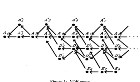
(9) 9. and call it the order of g at x_{0} is. The. .. and continuous.. surjective. projection, (f, x_{0}). sufficiently small,. In. mapping. fact,. let. $\varphi$ $\pi$. \mathcal{G}(\mathrm{R}, \mathrm{R})\backslash $\Sigma$_{\infty}\rightar ow \mathrm{N}. :. C^{\infty}(\mathrm{R}, \mathrm{R}). :. (C^{\infty}(\mathrm{R}, \mathrm{R}) \times \mathrm{R})\backslash $\pi$^{-1}($\Sigma$_{\infty}). \in. ,. \mathrm{R}. \times. \displaystle\mathrm{o}\mathrm{}\mathrm{d}_x0}\frac{df} x. and. defined. =n. K=[x0- $\epsilon$, x_{0}+ $\epsilon$], V=(x0- $\epsilon$, x0+ $\epsilon$). and set. by. \mathcal{G}(\mathrm{R}, \mathrm{R}). \rightarrow. .. f_{x0}\displaystyle\mapsto\mathrm{o}\mathrm{r}\mathrm{d}_{x_{0}\frac{df}{dx}. be the natural if. Then,. take $\epsilon$>0. we. ,. U=\{j^{n+1}g(x)\in J^{n}(\mathrm{R}, \mathrm{R})| |g^{(n+1)}(x)-f^{(n+1)}(x_{0})|< $\epsilon$\}, (g, x). then. W(n, K, U). \in. maps any open subset to any a. \overline{$\varphi$}. :. Then. .. we. Since. choose. we. n. Moreover $\varphi$ is. .. for any open set. $\epsilon$(x_{0}) \neq 0. \rightarrow. N.. Then \overline{$\varphi$} is. x^{n+1}. to the germ of. at 0. a. an. mapping,. open. vanishing dg. outside of. \mathrm{o}\mathrm{r}\mathrm{d}_{x_{0} \overline{dx}=\el. bijection.. In. fact,. if. .. The. a. ,. df. $\varphi$. and. where. $\epsilon$. is. neighbourhood. mapping. \mathrm{o}\mathrm{r}\mathrm{d}_{x0_{\overline{dx}. i.e.. (f, x_{0}). W of. neighbourhood. g(x)=f(x)+ $\epsilon$(x)(x-x_{0})^{l+1}. and. appropriate, then g\in W and. $\epsilon$. \overline{ $\varphi$}^{-1} : \mathrm{N}\rightar ow(\mathcal{G}(\mathrm{R}, \mathrm{R})\backslash $\Sigma$_{\infty})/\sim A. Next. \leq. that. satisfying. (\mathcal{G}(\mathrm{R}, \mathrm{R})\backslash $\Sigma$_{\infty})/\sim A. diffeomorphic. \displaystle\mathrm{o}\mathrm{}\mathfact, rm{d}_x\frac{dg} x. open subset. In. 0\leq\ell\leq $\varphi$(f_{x0})=\mathrm{o}\mathrm{r}\mathrm{d}_{x0_{\overline{dx}'}. differentiable function. of x_{0}. implies. df. \ell with. integer. \times V. an. =. n. $\varphi$ induces. then. f_{x0}. is. Moreover $\varphi$ is continuous and an open mapping. \square continuous, we see \overline{$\varphi$} is a homeomorphism.. .. is also. consider. we. \mathcal{G}(\mathrm{R}^{2}, \mathrm{R})=(C^{\infty}(\mathrm{R}^{2}, \mathrm{R})\times \mathrm{R}^{2})/\sim, the space of germs of real‐valued functions Then we have. Proposition 4.2 For tions are equivalent to. (1) (2). V/\sim A. set. For the. there exists. an. of points. If. one. call the we can. f. germ. :. (\mathrm{R}^{2}, x_{0}). U\in O of g in \mathcal{G}. the. following. condi‐. fulfilled,. [f_{x_{0}}]. .. We. Theorem 4.3 The. we. Then. quotient. see. f. :. (\mathrm{R}^{2}, x_{0})\rightarrow(\mathrm{R}, y_{0}). (simple). (or simple) if. 0‐modal. we. In. general,. 0 ‐modal. for. (or simple),. and also. a. have. space. space (Figure 1).. proof,. call. topological space (\mathcal{G}, \mathcal{O}) \in \mathcal{G} 0 ‐modal there exists an open finite neighbourhood denote by $\Sigma$_{NS}\subset \mathcal{G}(\mathrm{R}^{2}, \mathrm{R}) the set consisting of diffeomorphism classes Then \mathcal{G}(\mathrm{R}^{2}, \mathrm{R})\backslash $\Sigma$_{NS} designates the set consisting of diffeomorphism. non‐simple germs. classes of simple germs.. topology. ,. ∼. of. a. \mathcal{G}(\mathrm{R}^{2}, \mathrm{R}). \in. a. equivalence call a point g. O. ,. an. is. class. Let X be. (\mathrm{R}, y_{0}) f_{x0}. each other:. of conditions is. For the. \rightarrow. \mathrm{R}^{2}.. open neighbourhood V of f : (\mathrm{R}^{2}, x_{0}) \rightarrow (\mathrm{R}, y_{0}) in \mathcal{G}(\mathrm{R}^{2},\mathrm{R}) the finite set. equivalence class [f_{x_{0} ]\in \mathcal{G}(\mathrm{R}^{2}, \mathrm{R})/\sim A of f_{x_{0}} for the equivalence relation A, open neighbourhood of [f_{x0}] in \mathcal{G}(\mathrm{R}^{2}, \mathrm{R})/\sim A which consists of a finite number. There exists. quotient. a. on. (\mathcal{G}(\mathrm{R}^{2}, \mathrm{R})\backslash $\Sigma$_{NS})/\sim A. is. homeomorphic. to the ADE‐. [1].. set and. \mathcal{W}=\{W_{ $\mu$}\}. is. a. family of subsets of X Then topology generated by \mathcal{W}.. containing \mathcal{W} We call it the .. .. there exists the minimal.

(10) 10. Figure. Let. X=(X, \mathcal{O}_{X}). be. a. topological. 1:. ADE‐space. space, and Y. a. subset of X. \mathrm{y} of the form \mathrm{Y}\cap V for any open subset V\in \mathcal{O}_{X} of X O_{Y} , which is called the relative topology on Y. Let. X=(X, \mathcal{O}_{X}). the quotient. topology. be. a. on. X/\sim \mathrm{b}\mathrm{y} setting. topological. space, \sim \mathrm{b}\mathrm{e}. an. .. Then. .. we. equivalence. Then. get. a. we. collect subsets of. topological. relation. on. X. .. structure. The. we. give. \mathcal{O}_{X/\sim} :=\{U\subseteq X/\sim | $\pi$^{-1}(U)\in \mathcal{O}_{X}\}. Then. U\subseteq X/\sim \mathrm{i}\mathrm{s}. Let. open if and. X, Y be topological. subset U of Y , the inverse. only if $\pi$^{-1}(U). spaces. A. mapping f. f^{-1}(U). image. is open in X.. is. an. :. X\rightarrow \mathrm{Y} is called continuous if for any open. open subset of X.. A mapping $\varphi$ : X \rightarrow \mathrm{Y} is called a homeomorphism if $\varphi$ is one‐to one onto continuous mapping and the inverse mapping $\varphi$^{-1} is also continuous. If there is a homeomorphism from X to Y then we call X and \mathrm{Y} are homeomorphic. ,. Example 4.4 (1) \mathrm{L}\mathrm{e}\mathrm{t}\sim \mathrm{b}\mathrm{e} an equivalence relation on \mathrm{R} defined by the condition that x\sim x' if and only if x' x or x'= -x We give on \mathrm{R}/\sim the quotient topology from R. On the other hand we give the relative topology on the half line \mathrm{R}_{\geq 0} \{x \in \mathrm{R} | x \geq 0\} from R. The we see \mathrm{R}/\sim and \mathrm{R}_{\geq 0} are homeomorphic. (2) We define another equivalence relation \approx \mathrm{o}\mathrm{n}\mathrm{R} by that x\approx x' if and only if x=x'=0 or xx' \neq 0 The quotient set \mathrm{R}/\approx consists of two equivalence relations: \mathrm{R}/\approx \{[0] [1] \}. The quotient topology on \mathrm{R}/\ap rox \mathrm{i}\mathrm{s} given by \{\emptyset, \{[1]\}, \{[0], [1]\}\} This topological space can be indicated by the diagram: =. .. =. =. .. ,. .. \bullet\leftarrow\bullet. Let. ( $\Lambda$, \leq). be. a. partially ordered. set: A relation. v\leq v'. on a. set $\Lambda$ is defined and satisfies. that v\leq v, (v\leq v', v'\leq v\Rightarrow v=v') and (v\leq v', v' \leq v'' v\leq v is called saturated if, for any v \in V, v' \in $\Lambda$, v' \leq v implies v' \in V all saturated subsets of $\Lambda$ satisfies the condition of. from. the. ordering.. topology.. Then .. a. Then the. It is called the. subset. V\subseteq $\Lambda$. family \mathcal{O}_{ $\Lambda$} of topology induced.

(11) 11. Differentiable structure of. 5. In this section. we. introduce the method to. and their quotients. See also [18]. There are known several methods:. mapping. give. For. a. differentiable structure. instance,. differentials and Omoris method of ILB manifold method is. What. 5.1 Let. new. and easy to. are. apply compared. quotients. space. on. mapping. the Eells method based. (inverse. limit Banach. on. spaces. Frechet. manifold).. Our. with other known methods.. structures?. \{X_{ $\nu$}\}. be a family of sets. The family X_{ $\nu$} is supposed to consist of quotients of subspaces topological space, in particular a mapping space C^{\infty}(N, M) for manifolds N, M. To define a differentiable structure on each X_{ $\nu$} from \{X_{ $\nu$}\} it is sufficient to give a criterion, for each pair X_{\mathrm{v} , X_{$\nu$'}, X_{ $\nu$} and X_{$\nu$'} are diffeomorphic For that it is sufficient to give a criterion that a mapping $\Phi$ : X_{ $\nu$}\rightarrow X_{$\nu$'} is differentiable or not. Then, for example, how should we define that a given mapping $\Phi$ : C^{\infty}(N, M) \rightarrow C^{\infty}(L, W) ( L, W are manifolds) is differentiablei? Let $\Phi$ : C^{\infty}(N, M)\rightarrow C^{\infty}(L, W) be a mapping. Then, for each differentiable mapping f\in C^{\infty}(N, M) there corresponds a differentiable mapping $\Phi$(f) \in C^{\infty}(L, W) Now we propose to call $\Phi$ differentiablè if, for any differentiable family h_{ $\lambda$}\in C^{\infty}(N, M) $\Phi$(h_{ $\lambda$})\in C^{\infty}(L, W) is differentiable, where the fparameter $\lambda$ runs over a finite dimensional manifold $\Lambda$ In fact moreover we demand that $\Phi$ is continuous. As an ordinary term in global analysis and differential topology, we call h_{ $\lambda$} : N\rightarrow M, ( $\lambda$\in $\Lambda$) is a differentiable family if there exists a differentiable mapping H : $\Lambda$\times N\rightarrow M which satisfies h_{ $\lambda$}(x)=H( $\lambda$, x) for each ( $\lambda$, x)\in $\Lambda$\times N. Then the mapping h: $\Lambda$\rightarrow C^{\infty}(N, M) defined by h( $\lambda$)=h_{ $\lambda$} is called differentiable naturally. Then for $\Phi$(h_{ $\lambda$})\in C^{\infty}(L, W) we can take a differentiable mapping G : $\Lambda$\times L\rightarrow W with. of. a. ,. ,. .. ,. .. ,. $\Phi$(h_{ $\lambda$})(x'). respect. =. G( $\lambda$, x') ( $\lambda$, x') ,. \in L\times. Differentiability along. 5.2. W. .. Therefore. we can. take the derivative of. $\Phi$(h_{ $\lambda$}). with. to $\lambda$.. Consider another. example.. finite dimensional directions.. How to define the. differentiability of a functional $\Psi$ : C^{\infty}(L, W)\rightarrow $\Psi$(g) mapping g\in C^{\infty}(L, W) The function $\Psi$(g_{ $\lambda$}) of variable $\lambda$ is determined for finite dimensional differentiable family g_{ $\lambda$}\in C^{\infty}(L, W) $\lambda$\in $\Lambda$. Then we call a mapping $\Psi$ : C^{\infty}(L, W)\rightarrow \mathrm{R} differentiable if the function $\Psi$(g_{ $\lambda$}) is differentiable on $\lambda$ We regard each g_{ $\lambda$} \in C^{\infty}(L, W) as a point in the space C^{\infty}(L, W) Then the family of mapping g_{ $\lambda$} \in C^{\infty}(L, W) is regarded as a finite dimensional subspace in C^{\infty}(L, W) The family $\Psi$(g_{ $\lambda$}) is the restriction of $\Psi$ to there, and we look at the differentiability of $\Psi$(g_{ $\lambda$}) in the ordinary sense. The differentiability we are going to define may be called the differentiability along finite dimensional directions. \mathrm{R} ? The real value. is determined for each. .. ,. .. .. .. If $\Phi$. :. C^{\infty}(N, M). \rightarrow. C^{\infty}(L, W). and $\Psi$. :. C^{\infty}(L, W). \rightarrow. \mathrm{R}. are. differentiable then the. composition $\Psi$\circ $\Phi$ : C^{\infty}(N, M) \rightarrow \mathrm{R} is differentiable. If fact, for any differentiable family h_{ $\lambda$} \in C^{\infty}(N, M) we have ( $\Psi$\circ $\Phi$)(h_{ $\lambda$}) $\Psi$( $\Phi$(h_{ $\lambda$}) and $\Phi$ : C^{\infty}(N, M) \rightarrow C^{\infty}(L, W) is differentiable, we see $\Phi$(h_{ $\lambda$}) is differentiable on $\lambda$ Since $\Psi$ is differentiable, $\Psi$( $\Phi$(h_{ $\lambda$}) is differentiable, so is ( $\Psi$ 0 $\Phi$)(h_{ $\lambda$}) on $\lambda$. We have defined that $\Psi$ : C^{\infty}(L, W) \rightarrow \mathrm{R} is differentiable. On the other hand, since \mathrm{R} is identified with C^{\infty}(\{\mathrm{p}\mathrm{t}\}, \mathrm{R}) we can regard $\Psi$ : C^{\infty}(L, W) \rightarrow C^{\infty}(\mathrm{p}\mathrm{t}, \mathrm{R}) Then $\Psi$ is =. ,. .. ,. ..

(12) 12. differentiable in the. C^{\infty}(L_{:}W) $\Psi$(g_{ $\lambda$}) ,. sense. then H is differentiable.. Example. of the first definition.. is differentiable. on. $\lambda$. By definition,. 5.1 We define $\Psi$. system of coordinates. on. :. If $\Psi$. :. .. 2: The. First. we. start with the. case. that the. differentiable. for any differentiable. \rightarrow. \mathrm{R}. :. ,. by $\Psi$(f). :=. $\Psi$ is differentiable.. area. surrounded. mapping. N which will be identified with the space. Let N be. fact,. define H. Differential structure of manifold. 5.3. In. manifold,. S. family. g_{ $\lambda$} \in. $\Lambda$\times\{\mathrm{p}\mathrm{t}\}\rightar ow \mathrm{R} by H ( $\lambda$ pt) = $\Psi$(g_{ $\lambda$}) C^{\infty}(L, W)\rightarrow C^{\infty}(\{\mathrm{p}\mathrm{t}\}, \mathrm{R}) is differentiable.. we. C^{\infty}(S^{1}, \mathrm{R}^{2}). \mathrm{R}^{2} Then. Figure. .. by. a. \displaystyle \int_{S^{1} f^{*}(xdy). plane. ,. where x, y is the. curve.. quotients.. space is. a. C^{\infty}(\{\mathrm{p}\mathrm{t}\}, N). subset of. a. finite dimensional manifold. .. subset of N , and. a equivalence relation on S. Q play a role of test space Then the differentiability is introduced inductively as follows: (1) We call a mapping h : $\Lambda$\rightarrow S from a manifold to a subset of a manifold differentiable if the composed mapping h : $\Lambda$\rightarrow S\mapsto N is a differentiable mapping from the manifold $\Lambda$ to. Assume. $\Lambda$,. a. M and. are. a. \sim. also differentiable manifolds which. the manifold N.. (2). We call a mapping k : S\rightarrow Q from a subset of a manifold to a manifold differentiable if continuos, and for any differentiable mapping h : $\Lambda$\rightarrow S in the sense of (1), the composed mapping k\mathrm{o}h: $\Lambda$\rightarrow Q is a differentiable mapping from the manifold $\Lambda$ to the manifold Q. (3) We call a mapping \ell : S/\sim\rightarrow Q from a quotient of a subset of a manifold to a manifold differentiable if the composed mapping \ell 0 $\pi$ : S\rightarrow S/\sim\rightarrow Q is differentiable in the sense of k is. (2). (4). a mapping m : $\Lambda$ \rightarrow S/\sim from a manifold to a quotient of a subset of a differentiable if, for any differentiable mapping \ell : S/\sim \rightarrow Q in the sense of (3), the composed mapping \ell\circ m : $\Lambda$ \rightarrow Q is a differentiable mapping from the manifold $\Lambda$ to the manifold Q. More generally: (5) We call a mapping $\varphi$ : S/\sim\rightarrow T/\approx\leftarrow T\subseteq M from a quotient of a subset of a manifold to a subset of a manifold differentiable if $\varphi$ is continuous and, for any differentiable mapping \ell : T/\approx \rightarrow Q in the sense of (3), the composed mapping \ell 0 $\varphi$ : S/\sim \rightarrow Q is differentiable in. We call. manifold. sense of (3). (6) A mapping $\varphi$ : S/\sim\rightar ow T/\approx \mathrm{i}\mathrm{s} called a diffeomorphism if $\varphi$ is differentiable in the sense of (5), bijective, and the inverse mapping $\varphi$^{-1} : T/\approx \rightarrow S/\sim \mathrm{i}\mathrm{s} differentiable in the sense of (5). (7) The quotient spaces S/\sim and T/\approx are called diffeomorphic if there exists a diffeomor‐ phism $\varphi$ : S/\sim\rightarrow T/\approx.. the.

(13) 13. Remark 5.2 There is. different definition for the stage. a. is called differentiable if there exists. mapping \overline{k}. an. k Q satisfying \overline{k}|_{S} extensions of mappings on S our definition called a parametric‐minded definition. :. U. \rightarrow. =. .. ,. Example. 5.3. which acts. on. By. (Differentiable \mathrm{R}^{n}. structure. naturally. general theory,. the above. we. (2) (cf. [24]):. neighbourhood Compared with this. open. on. can. is based. orbifolds).. on. A. mapping k:S\rightarrow Q. U in N and. a. differentiable. definition which is based. parametrisations of S and. Let G be. endow with the. . finite. a. of. \mathrm{G}\mathrm{L}(n, \mathrm{R}). the. ordinary. subgroup. orbifold. \mathrm{R}^{n}/G. on. may be. differentiable structure.. Example relation. quotient space \mathrm{R}/\sim \mathrm{i}\mathrm{s} diffeomorphic to \mathrm{R}_{\geq 0} where \sim \mathrm{i}\mathrm{s} an equivalence by that x\sim x' if and only if x'=\pm x. : x^{2} is a diffeomorphism. For, $\varphi$ 0 $\pi$ : \mathrm{R} \rightarrow \mathrm{R}_{\geq 0}, \mathrm{R}/\sim \rightarrow \mathrm{R}_{\geq 0}, $\varphi$([x]) x^{2} is a continuous differentiable mapping by (1), we see $\varphi$ is a differentiable. 5.4 The. on. In fact $\varphi$. ( $\varphi$ 0 $\pi$)(x). ,. \mathrm{R} defined. =. =. mapping by (3). The inverse mapping is given by $\psi$ : \mathrm{R}_{\geq 0} \rightarrow \mathrm{R}/\sim, $\psi$(y) 1\sqrt{y}]. To see $\psi$ is differentiable, we check, based on (5), for any differentiable mapping \ell : \mathrm{R}/\sim \rightarrow Q, that l\mathrm{o} $\psi$ : \mathrm{R}_{\geq 0} \rightarrow Q is differentiable. By (3), \ell\circ $\pi$ : \mathrm{R} \rightarrow Q is differentiable. Since (\ell\circ $\pi$)(x) (\ell\circ $\pi$)(-x) we see there exists a differentiable mapping $\rho$ : \mathrm{R} \rightarrow Q with (\ell\circ $\pi$)(x)=p(x^{2}) Then (\ell\circ $\psi$)(y)=\ell([fy])=(\ell 0 $\pi$)(\sqrt{y})= $\rho$(y) Thus \ell\circ $\psi$ is differentiable. =. =. ,. .. .. \square. Example. 5.5 We. (x', y')=\pm(x, y) to. .. give. Then. the. equivalence. we see. \mathrm{R}^{2}.. relation∼on. \mathrm{R}^{2}/\sim \mathrm{i}\mathrm{s}. \mathrm{R}^{2} by that (x, y)\sim(x', y') if and only if to \mathrm{R}^{2} but \mathrm{R}^{2}/\sim \mathrm{i}\mathrm{s} not diffeomorphic. homeomorphic. mapping s:\mathrm{R}^{2}/\sim\rightar ow \mathrm{R}^{2}, s([(x, y)])=(x^{2}-y^{2},2xy) is a homeomorphism. However s diffeomorphism. Moreover we see that there exists no diffeomorphism between \mathrm{R}^{2}/\sim and \mathrm{R}^{2} To see that, suppose that there exist a differentiable mapping $\psi$ : \mathrm{R}^{2}\rightar ow \mathrm{R}^{2}/\sim and a differentiable mapping $\varphi$:\mathrm{R}^{2}/\sim\rightar ow \mathrm{R}^{2} satisfying $\psi$\circ $\varphi$=\mathrm{i}\mathrm{d}, $\varphi$\circ $\psi$=\mathrm{i}\mathrm{d} Since $\varphi$ 0 $\pi$ : \mathrm{R}^{2}\rightar ow \mathrm{R}^{2} The. is not. a. .. .. is differentiable and invariant under the transformation. (x, y). (-x, -y). \mapsto. ,. there exists. a. mapping $\rho$ \mathrm{R}^{3} \rightar ow \mathrm{R}^{2} satisfying ( $\varphi$ 0 $\pi$)(x, y) = $\rho$(x^{2} xy, y^{2}) Therefore there exists a differentiable mapping $\Phi$ : \mathrm{R}^{2}/\sim \rightarrow \mathrm{R}^{3} with ( $\Phi$\circ $\pi$)(x, y) (x^{2} xy, y^{2}) so with $\varphi$\circ $\pi$ $\rho$ 0 $\Phi$ 0 $\pi$ Since $\pi$ is a surjective, we have $\varphi$ $\rho$ 0 $\Phi$ Therefore id $\varphi$ 0 $\psi$ However the image of $\Psi$ := $\Phi$ 0 $\psi$ : \mathrm{R}^{2} \rightarrow \mathrm{R}^{3} is contained in $\rho$ 0 ( $\Phi$\circ $\psi$) : \mathrm{R}^{2} \rightarrow \mathrm{R}^{2} \{ (x^{2}, xy, y^{2}) | (x, y) \in \mathrm{R}^{2}\}= \{(X, \mathrm{Y}, Z) \in \mathrm{R}^{3} | XZ-\mathrm{Y}^{2} =0\} and thus \mathrm{r}\mathrm{a}\mathrm{r}\mathrm{k}_{0}$\Psi$ \leq 1 This differentiable. :. .. ,. =. =. =. .. .. ,. =. =. .. .. leads. a. contradiction.. \square. Example 5.6 (The differentiable structure of a quotient space by the complex conjugation) conj: \mathrm{C}^{n}\rightarrow \mathrm{C}^{n} conj (z)=\overline{z} be the complex conjugation. The quotient space C/conj is diffeomorphic to \mathrm{R}\times \mathrm{R}_{\geq 0} For \mathrm{C}^{2}/ conj, it is homeomorphic to \mathrm{R}^{4} and it is not diffeomorphic to \mathrm{R}^{4} Then we endow \mathrm{C}^{2}/ conj with the differentiable structure induced from the standard one on \mathrm{R}^{4} If we endow a differentiable structure on \mathrm{C}P^{2}/ conj in the same way as above, we see that \mathrm{C}P^{2}/ conj is diffeomorphic to the ‐sphere S^{4} (The theorem of Kuiper, Massey, Let. ,. .. .. .. .. Arnold.) 5.4 Let. Differentiable structures. N, M, L, P. on. mapping. be differentiable manifolds.. (finite dimensional). differentiable manifolds. space. Moreover, in respectively.. quotients.. this. section, $\Lambda$, Q always designate.

(14) 14. X\subseteq C^{\infty}(N, M) be a subset. Then, such a set X is a mapping space. (1) We call a mapping h : $\Lambda$ \rightarrow X differentiable if there exists a differentiable mapping (between manifolds) H: $\Lambda$\times N\rightarrow M satisfying H( $\lambda$, x)=h( $\lambda$)(x)\in $\Lambda$ l, ( $\lambda$\in $\Lambda$, x\in N) (2) We call a mapping k:X\rightarrow Q differentiable if Let. .. k is. continuous. mapping and, for any for any differentiable mapping h : $\Lambda$\rightarrow X in the composition k\circ h: $\Lambda$\rightarrow Q is a differentiable mapping between manifolds. (1), Now, \mathrm{i}\mathrm{f}\sim \mathrm{i}\mathrm{s} an equivalence relation on a mapping space X then we get the quotient space X/\sim Such a quotient space X/\sim \mathrm{i}\mathrm{s} called a mappings space quotient. Then the projection $\pi$ : X\rightarrow X/\sim \mathrm{i}\mathrm{s} defined by $\pi$(x)=[x] (the equivalence class of x ). (3) We call a mapping \ell : X/\sim\rightarrow Q differentiable if the composition l\circ $\pi$ : X\rightarrow Q with the projection $\pi$ is differentiable in the sense of (2). (4) We call a mapping m : $\Lambda$ \rightarrow X/\sim differentiable if, for any differentiable mapping \ell : X/\sim\rightarrow Q in the sense of (3), the composition \ell \mathrm{o}m : $\Lambda$\rightarrow Q is a differentiable mapping a. of. sense. the. ,. .. between manifolds. Lemma 5.7 in the. Proof: \ell\circ $\pi$. :. sense. If h: $\Lambda$\rightarrow X of (4).. is. differentiable. For any differentiable mapping \ell : differentiable in the sense of. X\rightarrow Q. differentiable. Hence $\pi$\circ h differentiable in. (5). in the. sense. of (1), $\pi$\circ h: $\Lambda$\rightarrow X/\sim is differentiable. X/\sim \rightarrow Q in the sense of (3), the composition (2). Therefore (\ell 0 $\pi$)\mathrm{o}h=\ell \mathrm{o}( $\pi$ \mathrm{o}h) : $\Lambda$\rightarrow Q is \square the sense of (4).. general, we call a mapping $\varphi$ : X/\sim\rightarrow Y/\approx from a mapping space quotient X/\sim mapping space quotient Y/\approx\leftarrow Y\subseteq C^{\infty}(L, P) differentiable if $\varphi$ is a continuous mapping and, for any differentiable mapping \ell:Y/\approx\rightarrow Q in the sense of (3), the composition \ell 0 $\varphi$ : X/\sim\rightarrow Q is differentiable in the sense of (3). (6) Then we call a mapping $\varphi$ : X/\sim\rightar ow \mathrm{Y}/\approx \mathrm{a} diffeomorphism if $\varphi$ is differentiable in the sense of (5), $\varphi$ is a bijection and the inverse mapping $\varphi$^{-1} : Y/\approx\rightarrow X/\sim \mathrm{i}\mathrm{s} also differentiable In. to another. in the. (7) a. sense. Then. of. (5).. we. call two. diffeomorphism. Lemma 5.8 The. $\varphi$. :. mapping. space. X/\sim\rightarrow Y/\approx \mathrm{i}\mathrm{n}. following. quotients X/\sim and Y/\approx diffeomorphic if there. the. sense. two conditions. are. of. exists. (6).. equivalent. to each other:. (i) $\varphi$ : X/\sim\rightarrow Y/\approx is differentiable in the sense of (5). (ii) $\varphi$ : X/\sim \rightarrow \mathrm{y}/\approx \dot{u} a continuous mapping and, for any differentiable mapping $\Lambda$\rightarrow X/\sim in the sense of (4), $\varphi$\circ m: $\Lambda$\rightarrow Y/\approx differentiable in the sense of (4).. m :. Proof: (i) \Rightarrow (ii): Let P:Y/\approx\rightarrow Q be a differentiable mapping in the sense of (3). By (i), l\mathrm{o} $\varphi$ : X/\sim\rightarrow Q differentiable in the sense of (3). Then (P\circ $\varphi$)\mathrm{o}m=P\mathrm{o}( $\varphi$\circ m) : $\Lambda$\rightarrow Q is a differentiable mapping. Therefore $\varphi$ \mathrm{o}m : $\Lambda$\rightar ow \mathrm{Y}/\ap rox \mathrm{i}\mathrm{s} a differentiable mapping in the sense. (4). (\mathrm{i}\mathrm{i})\Rightar ow (i) : For any differentiable mapping P:\mathrm{Y}/\approx\rightarrow Q in the sense of (3), we check that \ell\circ $\varphi$ : X/\sim \rightarrow Q is differentiable in the sense of (3), namely that (\ell 0 $\varphi$)0 $\pi$ : X \rightarrow Q is differentiable in the sense of (2). Then we check, for any differentiable h : $\Lambda$\rightarrow X in the sense of (1), that ((\ell\circ $\varphi$)\circ $\pi$)\circ h: $\Lambda$\rightarrow Q is differentiable. By 5.7, $\pi$\circ h: $\Lambda$\rightar ow X/\sim \mathrm{i}\mathrm{s} differentiable in the sense of (4). Therefore, by (ii), ( $\varphi$\circ $\pi$)\circ h= $\varphi$\circ( $\pi$\circ h) : $\Lambda$\rightar ow Y/\approx \mathrm{i}\mathrm{s} differentiable in the sense of (4). Hence \ell \mathrm{o}( $\varphi$ 0 $\pi$)\mathrm{o}h=((\ell 0 $\varphi$)\circ $\pi$)\mathrm{o}h : $\Lambda$\rightarrow Q is is a differentiable mapping. \square Thus $\varphi$ is differentiable in the sense of (5). of.

(15) 15. Lemma 5.9 For C^{\infty} in the. sense. Proof: By satisfies. of (1). the. \dot{u}. topology a. on. C^{\infty}(N, M). continuous. assumption, there exists. H( $\lambda$, x)=h( $\lambda$)(x). Take. .. a. ,. differentiable mapping h: $\Lambda$\rightarrow X\subseteq C^{\infty}(N, M). mapping.. an. a. differentiable mapping H : $\Lambda$ C^{\infty}(N, $\lambda$ f) of the form. open subset of. compact subset and U\subseteq J^{r}(N, M) is an open subset. Suppose, for a $\lambda$_{0} \in $\Lambda$, h($\lambda$_{0}) H|_{$\lambda$_{0}\times N} : N\times 1\mathrm{I}4 belongs to. K\subseteq N is. \times. N. \rightarrow. M which. W(r, K, U). ,. where. a. =. $\Lambda$\times N\rightarrow J^{r}(N, M) by jí H( $\lambda$, x)=j^{r}(H|_{ $\lambda$\times N})(x). Then. .. jí H. is. W(r, K.U). a. .. jí H : mapping in. Define. differentiable. particular it is continuous. From the assumption h($\lambda$_{0})\in W(r, K, U) (jí H)^{-1}(W(r, K, U)) an open neighbourhood of $\lambda$_{0}\times K Since K is compact, there exists an This means that $\lambda$_{0}\in open neighbourhood V of $\lambda$_{0} such that V\times K\subseteq ( jí H)^{-1}(W(r, K, U V \subseteq h^{-1}(W(r, K, U Therefore h^{-1}(W(r, K, U)) is open. Noting that h^{-1}(W(r, K, U)\cap the. ordinary. In. sense.. ,. is. .. W(r', K', U =h^{-1}(W(r, K, U))\cap h^{-1}(W(r', K', U , h^{-1}(\cup W_{ $\nu$})=\cup h^{-1}(W_{ $\nu$}). ,. we see. h is. continuous.. \square. Remark 5.10 Lemma 5.9 does not hold for. C^{\infty}(\mathrm{R}, \mathrm{R}). ,. consider the differentiable. Whitney. mapping h. C^{\infty}. For. topology.. \mathrm{R}\rightarrow C^{\infty}(\mathrm{R}, \mathrm{R}). :. example, in X by the differen‐ =. defined. tiable mapping H( $\lambda$, x) := $\lambda$ Then h(0) is identically 0 Its graph is \mathrm{R}\times 0\subset \mathrm{R}\times \mathrm{R} Then there exists an open set U containing \mathrm{R}\times 0 such that h^{-1}(W(U))=\{0\} Then W(U) is an .. .. .. .. open subset of. C^{\infty}(\mathrm{R}, \mathrm{R}). with respect to. Whitney. (2),. Remark 5.11 In the above definition condition that for any differentiable k\circ h: $\Lambda$\rightarrow Q is differentiable. In fact set. the. topology, while h^{-1}(W(U))=\{0\}\subset \mathrm{R} Whitney C^{\infty} topology.. C^{\infty}. is not open in R. Therefore h is not continuous in. continuity of h. mapping h. :. $\Lambda$. \rightarrow. is not. X in the. implied from just the (1), the composition. sense. X=\{1/n\}\cup\{0\}\subset \mathrm{R}=C^{\infty}(\{\mathrm{p}\mathrm{t}\}, \mathrm{R}) and \mathrm{Y}=\{0, 1\}=C^{\infty}(\{\mathrm{p}\mathrm{t}\}, \{0,1 by k(1/n)=1, k(0)=0 Then any differentiable mapping h: $\Lambda$\rightarrow X. Define k:X\rightarrow \mathrm{Y}. is. .. locally constant, and so is k oh: $\Lambda$\rightarrow Y Then k\circ h is differentiable, while k is not continuous. Thus, in the definition (2), we need the continuity of k. .. Properties.. 5.5. Lemma 5.12 Let M be. a. differentiable manifold.. Then M\dot{u}. Proof: Both $\varphi$ : M \rightarrow C^{\infty}(\{\mathrm{p}\mathrm{t}\}, M) $\varphi$(x)(\mathrm{p}\mathrm{t}) := x f (pt), are differentiable and inverse mappings to each ,. and $\psi$ other.. ,. diffeomorphic :. to. C^{\infty}(\{\mathrm{p}\mathrm{t}\}, M). C^{\infty}(\{\mathrm{p}\mathrm{t}\}, M) \rightarrow. M, $\psi$(f). .. :=. \square. (1) The identity mapping id: X/\sim \rightarrow X/\sim \dot{u} differentiable. X/\sim \rightarrow Y/\approx and g:Y/\approx\rightarrow Z/\equiv are both differentiable, then. Lemma 5.13. (2) If f g\mathrm{o}f. :. :. Proof: (1). is clear.. (2). Since. any differentiable mapping. mapping. Moreover we see. g\mathrm{o}f. the composition. X/\sim \rightarrow Z/\equiv is differentiable. f and Then,. g. are. continuous, gof is continuous. Let m: $\Lambda$\rightarrow X/\sim \mathrm{b}\mathrm{e} assumption, f\mathrm{o}m : $\Lambda$\rightar ow \mathrm{Y}/\ap rox \mathrm{i}\mathrm{s} a differentiable. from the. g\mathrm{o}(f\mathrm{o}m). =. (g\mathrm{o}f)\mathrm{o}m. :. $\Lambda$\rightar ow Z/\equiv \mathrm{i}\mathrm{s}. differentiable. Therefore. is differentiable.. (1) The quotient mapping $\pi$ : X \rightarrow X/\sim is differentiable. (2) f X/\sim\rightarrow \mathrm{y}/\approx is differentiable if and only if f\circ $\pi$ : X\rightarrow Y/\approx is differentiable.. Lemma 5.14 :. \square. A. mapping.

(16) 16. Proof: (1) That $\pi$ is continuous is clear. For any differentiable mapping \ell : X/\sim \rightarrow Q, : X\rightarrow Q is differentiable. Therefore $\pi$ is differentiable. (2) f is continuous if and only if is f\circ $\pi$ continuous. If f is differentiable, then f\circ $\pi$ is differentiable. Conversely, assume f\mathrm{o} $\pi$ is differentiable and take any differentiable mapping \ell : \mathrm{Y}/\approx\rightarrow Q. \ell\circ(f\circ $\pi$)=(P\mathrm{o}f)\circ $\pi$ : X\rightarrow Q \square is differentiable. Hence \ell \mathrm{o}f is differentiable. Thus f is differentiable. \ell\circ $\pi$. Lemma 5.15. C^{\infty}(N, M) Example. \displaystyle \int_{K}f(x)dx. N and N'. If. C^{\infty}(N', M'). and. are. are. 5.16 Let K \subset \mathrm{R} be. Then the. .. mapping. diffeomorp hic,\cdot and, diffeomorphic. a. M and M'. compact subset. Define I. I is differentiable. (in. the. sense. :. are. diffeomorphic,. C^{\infty}(\mathrm{R}, \mathrm{R}). \rightarrow. of the definition. \mathrm{R}. then. by I(f). =. (2)).. Product space.. 5.6. X\subseteq C^{\infty}(N, M) Y\subseteq C^{\infty}(L, P). For. ,. ,. we. set. X\times \mathrm{y}=\{F\in C^{\infty} (N \mathrm{I}\mathrm{I} L, M\mathrm{U}P) |F(N)\underline{\subseteq}M, F(L)\underline{\subseteq}P\}, where N II L is the where space. we. quotients. Example mapping. that. f(x). (f', g^{j}). \equiv. regarded. is. union of N and L. disjoint. (f, g). define. as a. Then identify X/\sim \times \mathrm{Y}/\approx with (X\times Y)/\equiv, by that f\sim f' and g \approx g' Thus the product of mapping mapping space quotient. .. .. mapping C^{\infty}(N, M)\times N\rightarrow M defined by (f, x)\mapsto f(x) is a differentiable that if f_{n} \rightarrow f, x_{n} \rightarrow x then f_{n}(x_{n}) \rightarrow f(x) (n\rightarrow \infty) and moreover differentiable both for f and x.. 5.17 The This is. means. ,. mapping $\Phi$ : C^{\infty}(N, M) \times C^{\infty}(M, L) \rightarrow C^{\infty}(N, L) defined by $\Phi$(f, g) differentiable mapping.. Lemma 5.18 The. g\circ f. is. a. =. Proof: By proposition 3.3, $\Phi$ is continuous. Suppose h : $\Lambda$ \rightarrow C^{\infty}(N, M) \times C^{\infty}(M, L) is a mapping. Suppose a differentiable mapping H : $\Lambda$\times ( N II M ) \rightarrow M\mathrm{U}L defined the differentiable mapping h Then we have H( $\Lambda$\times N)\subseteq M, H( $\Lambda$\times M)\subseteq L Set F :=H|_{ $\Lambda$\times N} differentiable. .. and G. :=. H|_{ $\Lambda$\times M}. Then. .. .. f_{ $\lambda$}(x). =. F( $\lambda$, x). and. g_{ $\lambda$}(f_{ $\lambda$}(x). =. g_{ $\lambda$}(F(x, $\lambda$). =. differentiable.. 6 We 6.1 Let. is \square. Examples give. several. examples. The space of. N=\{ $\alpha$, $\beta,\ \gamma$\}. discrete the. G( $\lambda$, F( $\lambda$, x)). topology.. be. as. the. applications. of. our. theory.. triangles.. a. 0‐dimensional manifold. Set M=. \mathrm{R}^{2}. .. The. mapping. correspondence f\mapsto(f( $\alpha$), f( $\beta$), f( $\gamma$)) Set. consisting of three points, endowed with the space C^{\infty}(\dot{N}, M) is diffeomorphic to \mathrm{R}^{6} by. .. T:=. { f\in C^{\infty}(N, M) |f( $\alpha$) f( $\beta$) f( $\gamma$) ,. ,. is not. collinear}..

(17) 17. Then T is the. of. space. which is identified with the open subset of. triangles. \mathrm{R}^{6}. \{(a\mathrm{i},a_{2};b_{\mathrm{i},b_{2;}\mathrm{c}\mathrm{i},c_{2})\in\mathrm{R}^{6}\Verta_{2}a_{1} b_{2}b_{1} c_{2}c_{1} \neq0\} Now. Then. going. we are. we. Euclid (\mathrm{R}^{2}). Here. :=. we assume. For. to. classify triangles by. denote the group of motions. { \left(\begin{ar y}{l 1&0 \ P&a b\ Q&c d \end{ar y}\right). the reflections. are. congruences. We set. \mathrm{R}^{2} by. on. (P, Q)\in \mathrm{R}^{2},. contained in. A=(x_{1}, x_{2})\in R^{2},. on. \mathrm{R}^{2}. the Euclidean metric.. Euclid(R2):. \left(\begin{ar y}{l a&b\ c&d \end{ar y}\right). is. a. orthogonal. matriX}.. Euclid(R2).. \left(\begin{ar y}{l \mathrm{l}&0 \ P&a b\ Q&c d \end{ar y}\right)\left(\begin{ar y}{l \mathrm{l}\ x_{1}\ x_{2} \end{ar y}\right)=\left(\begin{ar y}{l \mathrm{l}\ ax_{1}+bx_{2}+P\ cx_{1}+dx_{2}+Q \end{ar y}\right) Namely g(A) =g(x_{12}x). (ax_{1}+bx2+P, \mathrm{c}x_{1}+dx_{2}+Q). =. where S3 is the symmetry group of order three, which is define the action of G on C^{\infty}(N, M)\cong \mathrm{R}^{6} by. .. G=S_{3}\times \mathrm{E}\mathrm{u}\mathrm{c}\mathrm{l}\mathrm{i}\mathrm{d}(\mathrm{R}^{2}). Now set. equal. to. \mathrm{D}\mathrm{i}\mathrm{f}\mathrm{f}(N). in this. case.. ,. We. ( $\sigma$,g)(A, B, C)= $\sigma$(g(A),g(B), g(C)) the. permutation by. space. T/G. for. $\sigma$ ,. (A, B, C)\in \mathrm{R}^{6}. .. Then. is the space of congruence classes of. Theorem 6.1. The space. of T/G of congruence. T\subset C^{\infty}(N, M). is G ‐invariant. The. quotient. triangles. classes. of triangles. is. diffeomorphic. to. \mathrm{R}>0\times. C , where. C:=\{(x, y)\in \mathrm{R}^{2}|x^{2}-y^{3}\leq 0\} is the. narrower. classes. domain. of triangles. The part. corresponds. is. defined by the homeomorphic. \mathrm{R}>0 from \mathrm{R}>0. cusp to. In. curve.. particular the. \times C represents the parameter of. to the congruence classes of. the congruence classes of isosceles. ofT/G of congruence. space. \mathrm{R}^{2}\times \mathrm{R}_{\geq 0}=\{(x, y, z) |z\geq 0\}.. equilateral triangles, triangles.. similarity. The summit of C edge corresponds to. while the. Proof of Theorem 6.1: The. induces. mapping a. \mathrm{R}^{6}\supset T\ni(A, B, C)\mapsto(BC, CA, AB)\in (\mathrm{R}>0)^{3}. mapping $\Phi$_{1}. :. T/G. (a+b+c, ab+bc+ca, abc) of. \overline{V} Then. X is. .. we see. diffeomorphic. that $\Phi$ to. .. \rightarrow. (\mathrm{R}_{>0})^{3}/S_{3}. .. Then V induces. :. :=\overline{V}0$\Phi$_{1} : T/G\rightarrow X. \mathrm{R}>0\times C.. (\mathrm{R}_{>0})^{3} \rightarrow (\mathrm{R}_{>0})^{3} by V(a, b, c) (\mathrm{R}>0)^{3}/S_{3}\rightarrow(\mathrm{R}>0)^{3} Let X be the image. Define V. \overline{V}. :=. :. .. is. a. diffeomorphism.. Moreover. we see. that \square.

(18) 18. Diffeomorphism. 6.2. Let N be N is. on. groups.. compact manifold without boundary. Then the group \mathrm{D}\mathrm{i}\mathrm{f}\mathrm{f}^{\infty}(N) of diffeomorphisms topological group in the c\infty topology. Moreover the composition m:\mathrm{D}\mathrm{i}\mathrm{f}\mathrm{l}^{\infty}(N)\times. a. a. \mathrm{D}\mathrm{i}\mathrm{f}\mathrm{l}^{\infty}(N)\rightar ow \mathrm{D}\mathrm{i}\mathrm{f}\mathrm{l}^{\infty}(N) m( $\varphi$, $\psi$)= $\psi$\circ $\varphi$ ,. differentiable.. are. Thus,. in this sense,. and the inverse. \mathrm{D}\mathrm{i}\mathrm{f}\mathrm{f}^{\infty}(N). is. i:\mathrm{D}\mathrm{i}\^{E}^{\infty}(N)\rightar ow \mathrm{D}\mathrm{i}\mathrm{f}\mathrm{l}^{\infty}(N) i( $\varphi$)=$\varphi$^{-1} ,. regarded. as. infinite dimensional Lie. an. group.. The space of knots.. 6.3. The space \mathrm{E}\mathrm{m}\mathrm{b}(S^{1}, \mathrm{R}^{3}) \subset C^{\infty}(S^{1}, \mathrm{R}^{3}) is an open subset. Set G :=\mathrm{D}\mathrm{i}\mathrm{f}\mathrm{f}^{\infty}(S^{1}) \times \mathrm{D}\mathrm{i}\mathrm{f}\mathrm{f}^{\infty}(\mathrm{R}^{3}) Then the group G acts on C^{\infty}(S^{1}, \mathrm{R}^{3}) by ( $\sigma$, $\tau$)f :=Tofo $\sigma$^{-1} Then \mathrm{E}\mathrm{m}\mathrm{b}(S^{1},\mathrm{R}^{3}) is G‐invariant. Thus G acts also on \mathrm{E}\mathrm{m}\mathrm{b}(S^{1}, \mathrm{R}^{3}) .. .. .. Proposition. 6.2. \mathrm{E}\mathrm{m}\mathrm{b}(S^{1}, \mathrm{R}^{3})/G. The quotient space. nite discrete space.. We need of. an. If the. a. might claim that all global and concrete. knots. are. equal,. from the. is. diffeomorphic. viewpoint. to the. countably infi‐. of differentiable. condition to define the trivial knotsuch. as. being. structure; the. we. boundary. embedded disk. we. of knots. \mathrm{I}\mathrm{m}\mathrm{m}(S^{1}, \mathrm{R}^{3}) of immersions, instead of the space of embeddings, then \mathrm{I}\mathrm{m}\mathrm{m}(S^{1}, \mathrm{R}^{3})/G is not a discrete space. The Vassiliev invariant ([28][29]). take the space. quotient. space. be understood. can. as an. invariant constructed from the. space \mathrm{E}\mathrm{m}\mathrm{b}(S^{1}, \mathrm{R}^{3})/G into the non‐discrete space By the same idea, consider the open subset. Gen. (S^{1}, \mathrm{R}^{2}). :=. \mathrm{I}\mathrm{m}\mathrm{m}(S^{1}, \mathrm{R}^{3})/G.. embedding of. the discrete. { f\in C^{\infty}(S^{1},\mathrm{R}^{2})|f is generic}. of the space C^{\infty}(S^{1}, \mathrm{R}^{2}) of parametric plane curves. Here a plane curve f : S^{1}\rightarrow \mathrm{R}^{2} is called generic if f is an immersion and its self‐intersections are only transversal intersections. Then the group G. :=\mathrm{D}\mathrm{i}\mathrm{f}\mathrm{l}^{\infty}(S^{1})\times \mathrm{D}\mathrm{i}\mathrm{f}\mathrm{f}^{\infty}(\mathrm{R}^{2}). Proposition. 6.3. The. quotient. acts. space Gen. discrete space.. on. C^{\infty}(S^{1}, \mathrm{R}^{2}). and Gen (S^{1}, \mathrm{R}^{2}) is G ‐invariant.. (S^{1}, \mathrm{R}^{2})/G is diffeomorphic to the. countably infinite. Contrarily \mathrm{I}\mathrm{m}\mathrm{m}(S^{1}, \mathrm{R}^{2})/G is not discrete. The Arnold invariant [2] can be understood an invariant constructed by means of the embedding of the discrete space Gen (S^{1}, \mathrm{R}^{2})/G. into the non‐discrete space. 6.4. Superspace. Let N be. a. \mathrm{I}\mathrm{m}\mathrm{m}(S^{1}, \mathrm{R}^{2})/G.. of Riemannian structures.. differentiable manifold of dimension. \mathcal{R}_{N}. :=. {the. n. .. The space. Riemannian metrics. on. N}. be regarded as a mapping space. In fact, a Riemannian metric on N determines, by definition, to each point x\in N a positive definite symmetric bilinear form g_{x} : T_{x}N\times T_{x}N\rightarrow \mathrm{R} depending on x in a differentiable way. It is given by a differentiable section g : N \rightarrow T^{*}NT^{*}N which possesses the positivity. Thus we can regard as R_{N}\subset C^{\infty}(N, T^{*}NT^{*}N) where T^{*}NT^{*}N means the tensor product of cotangent bundle T^{*}N over N. can. ,.

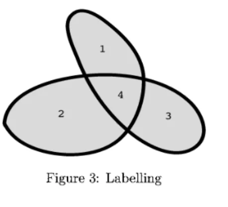
(19) 19. Now the. diffeomorphism. group. \mathrm{D}\mathrm{i}\mathrm{f}\mathrm{f}(N). acts. on. \mathcal{R}_{N} naturally. The quotient. space. (orbit. space) S_{N}:=\mathcal{R}_{N}/\mathrm{D}\mathrm{i}\mathrm{f}\mathrm{f}(N) is the space of. of N. isometry. classes of Riemannian structures. N and is called the super space. on. ([12][6]).. The. $\pi$^{-1}([g]). projection $\pi$ : \mathcal{R}_{N}\rightar ow \mathcal{S}_{N} is differentiable. For each isometry class [g] \in \mathcal{S}_{N} the fibre is diffeomorphic to the quotient space \mathrm{D}\mathrm{i}\mathrm{f}\mathrm{f}(N)/\mathrm{I}\mathrm{s}\mathrm{o}\mathrm{m}(N,g) of \mathrm{D}\mathrm{i}\mathrm{f}\mathrm{f}(N) by the isometry ,. group Isom (N,. g). of. (N, g). .. Theorem 6.4 Let N=S^{1}. \mathrm{R}_{>0} corresponds. .. to the total. Then. S_{S^{1}} is diffeomorphic to \mathrm{R}>0 and therefore to R. The space lengths of the one‐dimensional Riemannian manifolds (S^{1}, g) .. One of. interesting problem is to determine the superspace \mathcal{S}_{N} for a general N In the \dim N\geq 2 the space S_{N} turns out to be infinite dimensional. For example, in the case \dim N=2 the Gaussian curvature K:N\rightarrow \mathrm{R} on N gives a functional moduli on S_{N}. By the way, among the Riemannian metrics on N= S^{2} the round sphere, namely, the round sphere in the Euclidean \mathrm{R}^{3} seems to be distinguished. Then we are led to the following .. case. ,. ,. ,. conjecture: For the standard metric g_{0} on S^{2} , if (S_{S^{2}}, [g0]) and another (\mathcal{S}_{S^{2}}, [g]) morphic, then [g_{0}]=[g] , namely g is isometric to the standard metric g_{0}.. The. 6.5. symplectic. \mathrm{E}\mathrm{m}\mathrm{b}(S^{1},\mathrm{R}^{2}). Let. \subset. plane. Let ture. Symp (\mathrm{R}^{2}). moduli space of. C^{\infty}(S^{1}, \mathrm{R}^{2}). plane. curves.. be the space of differentiable. be the group of. locally diffeo‐. are. diffeomorphisms preserving. simple. closed. the standard. curves on. symplectic. the. struc‐. $\omega$_{0}=dx\wedge dy.. The group. H=\mathrm{D}\mathrm{f}\mathrm{f}\mathrm{i}(S^{1})\times \mathrm{S}\mathrm{y}\mathrm{m}\mathrm{p}(\mathrm{R}^{2}). acts. namely, by ( $\sigma$, $\tau$)f := $\tau$ \mathrm{o}f\mathrm{o}$\sigma$^{-1} quotient symplectomorphism classes of simple closed .. The. of. the space Emb (S^{1}, \mathrm{R}^{2}) in the natural way, space \mathrm{E}\mathrm{m}\mathrm{b}(S^{1}, \mathrm{R}^{2})/H is regarded as the space on. curves.. Proposition Ớ.5 The quotient space \mathrm{E}\mathrm{m}\mathrm{b}(S^{1},\mathrm{R}^{2})/H \mathrm{R}_{>0} corresponds to the area surrounded by curves. We consider. again. the open subset in. Gen (S^{1}, \mathrm{R}^{2}). :=. is. diffeomorphic. to. \mathrm{R}_{\geq 0}. .. The space. C^{\infty}(S^{1}, \mathrm{R}^{2}) :. { f\in C^{\infty}(S^{1}, \mathrm{R}^{2}) |f. is. generic}.. The group H=\mathrm{D}\mathrm{f}\mathrm{f}\mathrm{i}(S^{1})\times \mathrm{S}\mathrm{y}\mathrm{m}\mathrm{p}(\mathrm{R}^{2}) acts also on Gen (S^{1}, \mathrm{R}^{2}) Also another group G=\mathrm{D}\mathrm{i}\mathrm{f}\mathrm{f}(S^{1}) \times \mathrm{D}\mathrm{i}\mathrm{f}\mathrm{f}^{+}(\mathrm{R}^{2}) acts on Gen (S^{1}, \mathrm{R}^{2}) , where .. the group consisting of orientation preserving diffeomorphisms on For an f\in \mathrm{G}\mathrm{e}\mathrm{n}(S^{1}, \mathrm{R}^{2}) consider the G‐orbit G\cdot f through f. \mathrm{R}^{2}.. .. \mathrm{D}\mathrm{i}\mathrm{f}\mathrm{f}^{+}(\mathrm{R}^{2}). The group acts. on. is. G\cdot f.. The image f(S^{1}) of a generic mapping f : S^{1}\rightarrow \mathrm{R}^{2} divides \mathrm{R}^{2} into several regions. We put labels on bounded regions (Figure 3). Then for each f'\in G\cdot f , the bounded regions divided. by g'(S1) Then and that. have induced labels.. we $\tau$. define,. We call the curve. f.. for. f', f''\in G\cdot f, f'\sim f'' if there exists ( $\sigma$, $\tau$)\in H such that f''= $\tau$\circ f'\circ$\sigma$^{-1}. preserves the. quotient. labellings. space. A4(f) :=(G\cdot f)/\sim. the. symplectic moduli. space of the. plane.

(20) 20. Figure. symplectic moduli space \mathcal{M}(f) (G\cdot f)/\sim of a generic plane curve to (\mathrm{R}>0)^{r} therefore it is diffeomorphic to \mathrm{R}^{r} where r is the number of regions surrounded by f(S^{1}). Proposition 6.6 f is diffeomorphic bounded. Labelling. 3:. The. =. ,. ,. .. The space. (\mathrm{R}_{>0})^{r} corresponds. moduli spaces for. singular. more. to. areas. curves. of bounded domains. The structure of. is studied in. symplectic. [18].. References [1]. V.I.. [2]. V.I.. Arnold, Normal forms of functions near degenerate cntical points, Lagrange singularities, Funct. Anal. Appl., 6 (1972), 254‐272. Arnold, Topological. Invariants. of. Plane Curves and. Caustics,. the. Weyl. groups. Univ. Lect. Series. A_{k}, D_{k}, E_{k}. ,. and. 5, Amer. Math.. Soc. 1994.. [3]. V.I.. [4]. V.I.. [5]. D.. Arnold, Givental, Symplectic geometry, in Dynamical systems, IV, 1‐138, Encyclopaedia Math. Sci., 4, Springer, Berlin, (2001).. Arnold, V.V. Goryunov, O.V. Lyashko, V.A. Vasilev, S?ngularity Theory II. Classification and Ap‐ plications, Encyclopaedia of Math. Sci., Vol. 39, Dynamical System VIII, Springer‐Verlag (1993). Bennequin,. Entrelacements et. (Schnepfenried, 1982), Astérisque.. [6]. J.‐P.. Bourguignon,. (1975),. [7]. J.W.. Une. équations. de. 107‐108. (1983),. stratification. de. Pfaff,. lespace. Third. Schnepfenried geometry conference,. Vol. 1. 87‐161.. des structures. Riemanniennes, Compositio Math.,. 30. 1‐41.. Bruce,. T.. Gaffney, Simple singularities of mappings C, 0\rightar ow \mathrm{C}^{2}, 0, J. London Math. Soc.,. 26. 465‐474.. [8] Brylinski, Loop Spaces,. Characteristic Classes and Geometric. Quantization,. Progress. in. (1982),. Math., 107,. Birkhäuser 1993.. [9]. [10]. J.. Damon, The unfolding and determinacy theorems for subgroups of Soc., vol.50, No. 306, Amer. Math. Soc. (1984). W.. A and. K, Memoirs Amer. Math.. Domitrz, S. Janeczko, M. Zhitomirskii, Relative Poincaré lemma, contractibility, quasi‐homogeneity fields tangent to a singular varietyỳ Preprint.. and vector. [11]. Y.. Eliashberg, Contact 3‐manifolds twenty. 42. (1992),. no.. years since J. Martinets. work, Ann. Inst. Fourier (Grenoble). 1‐2, 165‐192.. [12] A.E.Fischer, Resolving. the. singularities. in the space. of Riemannian geometmes,. J. Math.. 27. (1986),. 113. (1993),. Phys.,. 718‐738.. [13]. C.G.. Gibson, C.A. Hobbs, Simple singularities of space. 297‐310.. curves,. Math. Proc. Camb. Phil.. Soc.,.

(21) 21. [14]. A.B.. Givental, Singular Lagrangian. Sovrem. Probl. Mat.,. [15]. M.. [16]. G.. varieties and their. (Contemporary. and. Lagrangian mappings,. Lagrange. stauilities. in. Itogi. Mathematics) 33, VITINI, (1988),. Stable mappings and their. Golubitsky, V. Guillemin, Springer‐Verlag, 1973. Ishikawa, Symplectic. Problems of. Nauki. Tekh., Ser.. pp. 55‐112.. Graduate Texts in. singularities,. of open Whitney umbrellas,. Invent.. math.,. Math., 14,. 12 $\epsilon$-2. (1996),. 215‐234.. [17] [18]. G. Ishikawa, of. Infinitesimal deformations Mathematics, 9‐1 (2005), 133‐166.. G.. and stabilities. of singular Legendre submanifolds, Asian Journal. Ishikawa, Global classification of curves on the symplectic plane, Complex Singularities, Sao Carlos, 2006, Contemporary. in. Real and. (2008), [i9]. G. of. [20]. Proceedings of the IX Workshop on 459, Amer. Math. Soc.,. Mathematics. pp. 51‐72.. Ishikawa, S. Janeczko, Symplectic bifurcations of plane Math., 54 (2003), 73‐102.. curves. and. vsotropic liftings, Quarterly Journal. A.. Kumpera, C. Ruiz, Sur Ìéquivalence locale des systèmes de Pfaff en drapeau, Equations and Related Topics, $\Gamma$ Gherardelli ed., Inst. Alta Math., Rome (1982), pp. .. [21] [22] [23]. [24]. Mather, Stability of C^{\infty} mappings. J.N.. (1969), J.N.. IJ :. III:. Finitely determined. IV: Class \ellfication. of. Montgomery,. (2001),. [27]. P.. map‐germs, Publ. Math.. M.. Zhitomirskii,. Geometrec. stable germs. Princeton Univ. Press. of Subreemannian Geometry, Their Montgomery, [25] Surveys and Monographs, vol. 91, Amer. Math. Soc., (2002). A Tour. R.. approach. by. [28].. V.A.. [29]. V.A.. Sci.. Math.,. 89. I.H.E.S.,. 35. to Goursat. \mathrm{R}. algebras,. Publ. Math.. (1997).. Geodesics and. flags,. Applications,. Anii. Inst. H.. Mathematical. Poincaré,. 18−4. Dynamical. and. 459‐493.. Mormul, Goursat flags: Classification of codimension‐one singularities,. Control. of. Infinitesimally stability implies stability, Ann.. Milnor, Topology from differentiable viewpoint,. R.. [26]. \mathrm{e}\mathrm{r}\mathrm{e}. 127‐156.. J.N. Mather, Stability of C^{\infty} mappings I.H.E.S., 37 (1970), 223‐248. J.. Monge‐Am. 254‐291.. Mather, Stability of c\infty mappings. (1968),. In. 201‐266.. Systems,. \not\in-3. (2000),. Journal of. 311‐330.. Vassiliev, Knot invariants Publishing, 1995.. and. singularity theory, Singularity theory (Trieste, 1991), 904‐919,. Vassiliev, Complements of Discriminants of Smooth Maps: Topology Edition, Trabsl. Math. Mono. vol. 98, Amer. Math. Soc. 1994.. and. [30]. C.T.C. Wall, Finite determinacy. Soc.,. [31]. M.. [32]. M. Zhitomirskii, Relative Darbouc theorem for singular manifolds Math., 57\triangleleft (2005) 1314‐1340.. of smooth. Zhitomirskii, Germs of integral Preprint NI00043‐SGT, (2000).. curves. map‐germs,. in contact. Bull. London Math.. 3‐space, plane and. Revised. Apphcations, 13. space curves,. and tocal contact. (1981),. World. 481‐539.. Isaac Newton Inst.. algebra_{J}. Canad. J.. Goo ISHIKAWA. Department of Mathematics, \mathrm{E} ‐mail. :. Hokkaido. University, Sapporo 060‐0810, JAPAN.. ishikawa@math.sci.hokudai.ac.jp. \mathrm{J}\mathrm{b}^{\backslash}\^{E}_{$\lambda$}\mathrm{a}_{-}\mathrm{x}\ovalbox{\t \smal REJECT}. .. pa \ovalbox{\t smal REJ CT} Ữf \ovalbox{\t smal REJ CT} ee. H. \mathb {H}\rflo r H $\beta$.

(22)