Explicit and direct representations of the solutions of nonlinear simultaneous equations (Applications of Reproducing Kernels)

(1)

Explicit

and

direct

representations of the

solutions

of

nonlinear

simultaneous equations

Masato

Yamada and

Saburou Saitoh

Abstract

In this paper we shall give practical, numerical and explicit

rep-resentations of inverse mappings of n-dimensional mappings (of the

solutions of n-nonlinear simultaneous equations) and show their

nu-merical experiments by using computers. We derive those concrete

formulas from very general ideas for the representation of the inverse

functions.

Keywords: Inverse function, inverse mapping, integral transform, integral representation, Green-Stokes formula, singular integral, fundamental

solu-tion, reproducing kernel, Sobolev space, non-linear mapping, general

non-linear equation.

MathematicsSubject

_{Classification}

(2000): Primary$93B30,93C10,35A35$

1 Introduction

The 2nd author of this paper considered that for any mapping $\phi$ from

an

arbitrary abstract set into

an

arbitrary set, he tried to consider the

represen-tation of the inversion $\phi^{-1}$ in terms of the direct mapping $\phi$ and he obtained

somesimpleconcrete formulas from

some

general ideas in ([1]). In this paper, from its general ideas, we shallgive practical representation formulasofsome

general functions. Here, weshallgive furthermoresome general methods and

ideas for the inversion formulas for

some

general non-linear mappings. We

shall first state the principles for

our

methods for the representations of

(2)

We shall consider

some

representation of the inversion $\phi^{-1}$ in terms of

some

integral form-at this moment,

we

shall need

a

natural assumption for

the mapping $\phi$ . Then, weshall transform the integral representation by the

mapping $\phi$ to the original space that is the defined domain of the mapping $\phi$. Then,

we

will be able to obtain the representation of the inverse $\phi^{-1}$

in terms of the direct mapping $\phi$

.

In [1], we considered the representation

of the inverse $\phi^{-1}$ in

some

reproducing kernel Hilbert spaces, and in [4],

we

consideredthe representations of the inverse $\phi^{-1}$ for

a

very concretesituation

and wegaveavery fundamentalrepresentation ofthe inversefor some general

functions

on

1 dimensional spaces.

Indeed, note that

$K(y_{1}, y_{2})= \frac{1}{2}e^{-1y-y|}12$ _{$y_{1},$} $y_{2}\in[\mathcal{A}, B]$ (1)

is the reproducing kernel for the Sobolev Hilbert space $H_{K}$ whose members

arereal-valued andabsolutelycontinuous functionson $[A, B]$ andwhose inner

product is given by

$(f_{1}, f_{2})_{H_{K}}= \int_{A}^{B}(f_{1}’(y)f_{2}’(y)+f_{1}(y)f_{2}(y))dy+f_{1}(A)f_{2}(A)+f_{1}(B)f_{2}(B)(2)$

([2]).

For

a

function $y=f(x)$ that is of $C^{1}$ class and

a

strictly increasing

function and $f’(x)$ is not vanishing on $[a, b](f(a)=A, f(b)=B)$, of course,

the inverse function $f^{-1}(y)$ is a single-valued function and it belongs to the

space $H_{K}$ and from the reproducing property, we obtain the representation,

for any $y_{0}\in[f(a), f(b)]$

$f^{-1}(y_{0})=(f^{-1}(\cdot),$ $K(\cdot, y_{0}))_{H_{K}}$

$= \int_{(a)}^{f(b)}((f^{-1})’(y)K_{y}(y, y_{0})+f^{-1}(y)K(y, y_{0}))dy$

$+aK(f(a), y_{0})+bK(f(b), y_{0})$. (3)

From this representation, we obtained in $([4|)$ the very simple representation

(3)

Furthermore, by using the several reproducing kernel Hilbert spaces from [2] as in (3), we calculated similarly with the related assumptions, however, surprisingly enough,

we

obtain the same formula (4). For the formula (4),

we note directly that we do not need any smoothness assumptions for the

function $f(x)$, indeed,

we

need only the strictly increasing assumption. The

assumption of integrability does not, even, need for the formula (4).

Now, we would like to obtain some multi-dimensional versions. At this moment, it seems that we can not find some simple representations

as

in (3) by some concrete known reproducing kernels for some general domains, and

indeed,

we

know the reproducing kernels only for special domains and for

special reproducing kernel Hilbert spaces.

In order to consider

some

general integral representations for

some

general

functions, we shall recall the fundamental facts:

We can represent afunction $f$ in termsofthe delta function $\delta$ in the form

$f(q)=/Df(p)\delta(p-q)dp$ (5)

in

some

domain, symbolically. Meanwhile, a fundamental solution $G(p-q)$ for some linear differential operator $L$ is given by the equation, symbolically

$LG(p-q)=\delta(p-q)$. (6)

So, from (5)

we

obtain the representation

$f(q)=/Df(p)LG(p-q)dp$

.

(7)

Then, we can obtain the representation symbolically, by using the Green-Stokes formula, for

some

adjoint operator $L^{*}$ for $L$,

$f(q)=/D^{L^{*}f(p)G(p-q)dp}+$

some

boundary integrals. (8)

We shall firstly

use

this type representation. In this approach,

we

will meet

thesingular integral representation in thefirst termof(8), however, if$G(p-q)$

is integrable, then by a simple regularization for $G(p-q)$ we will be able to

realize the representation in numerical treatments. In the separate paper

[3]

we

discussed the natural regularization in the form, for example, for the

singularity

(4)

we

consider the regularization

$\frac{1}{(|x-y|+\delta)^{\alpha}}$

for a small $\delta$ and

we

considered their

error

estimates.

We

are

interested in

some

very concrete results that may be realized by

computers. So,

we

considered veryconcrete

cases

in the 2 dimensionalspaces.

It

seems

that the results will depend on dimensions, domains and functions

spaces dealing with.

In [6], we considered the following typical problem:

Let $D\subset R^{2}$ be a bounded domain with a finite number of piecewise $C^{1}$

class boundary components. Let $f$ be

a

one-to-one $C^{1}$ class mapping from

$\overline{D}$

into $R^{2}$ and

we

assume

that its Jacobian _$J(x)$ is positive

on

$D$. We shall

represent $f$ as follows:

$y_{1}=f_{1}(x)=f_{1}(x_{1}, x_{2})$

$y_{2}=f_{2}(x)=f_{2}(x_{1}, x_{2})$ (9)

and the inverse mapping $f^{-1}$ of $f$

as

follows:

$x_{1}=(f^{-1})_{1}(y)=(f^{-1})_{1}(y_{1}, y_{2})$

$x_{2}=(f^{-1})_{2}(y)=(f^{-1})_{2}(y_{1}, y_{2})$

.

(10)

Then, we represented

$(\begin{array}{l}(f^{-1})_{1}(y^{*})(f^{-1})_{2}(y^{*})\end{array})$ (11)

in terms of the direct mapping (9).

Ofcourse, we are interested in some numerical and practical solutions of

the non-linear simultaneous equations (9) and

we

obtained

Proposition 1 $([6J)$ For the mappings (9) and (10) with (11),

we

obtain the

representation,

_for

any $y^{*}=(y_{1}^{*}, y_{2}^{*})\in f(D)$,

$(_{(f^{-1})_{2}(y^{*})}^{(f^{-1})_{1}(y^{*})})= \frac{1}{2\pi}\oint_{\partial D}(\begin{array}{l}x_{1}x_{2}\end{array})d$Arctan $\frac{f_{2}(x)-y_{2}^{*}}{f_{1}(x)-y_{1}^{*}}$

$- \frac{1}{2\pi}\int/D\frac{1}{|f(x)-y^{*}|^{2}}$adj$J(x)(\begin{array}{ll}f_{1}(x)- y_{1}^{*}f_{2}(x)-y_{2}^{*} \end{array})dx_{1}dx_{2}$

.

(12)

(5)

In this paper, we shall first give the natural versionfor the 3 dimensional

case by using the well-known Poisson integral formula and in the last,

sur-prisingly enough we shall give

some

unified and natural inversion formulas

for the general dimensions that

are

better than the formula derived from the

Poisson integral formula.

2 3-dimensional formula derived from

the

Pois-son

integral formula

Let $D$ be a bounded domain in $R^{3}$ with a finite number of $C^{1}$ boundary

components $\partial D$. Let _$f$ be a

one

to one $C^{2}$ class mapping of $D$ onto $f(D)$ in

$R^{3}$ with

sense

preserving and we

assume

that its Jacobian is positive on $D$.

We set

$y=f(x)=(f_{1}f_{3}f_{2}(((xxx))))=(\begin{array}{ll}x_{3}f_{1}(x_{1},x_{2},) f_{2}(x_{1},x_{2},x_{3}) f_{3}(x_{1},x_{2} x_{3})\end{array})$

and its inversion $f^{-1}$

as

follows:

$x=(f^{-1})(y)=(\begin{array}{l}(f^{-1})_{1}(y)(f^{-1})_{2}(y)(f_{3}^{-1})_{3}(y)\end{array})=((((f^{-1}f^{-1}f^{-1})_{2})_{3})_{1}(((y_{1}y_{1}y_{1}’ y_{2}y_{2}y_{2},y_{3}y_{3}y_{3}\})$

.

Let $\Delta=\overline{\partial}y_{1}\partial^{2}T+\cdots+\frac{\partial^{2}}{\partial y_{n}^{2}}$ and $\frac{\partial}{\partial}ux(x)$ be the Jacobian of $y=(y_{1}, \cdots, y_{n})$

with respect to$x=(x_{1}, \cdots, x_{n})$

.

For a matrix $A$, let $(A)_{i}$ be the $i$ low vector

of $\mathcal{A}$ and

$(A)_{ij}$ the $i,j$ element of $A$

.

We set the vector fields

$S_{i}(x)= \sum_{j=1}^{3}\frac{adj({}^{t}(\partial_{x}\partial A(x))(\partial\partial Ax(x))_{ij}}{\det(g_{(X))}}\frac{\partial}{\partial x_{j}}$ (13)

$T_{i}(x)= \frac{x_{i}}{|y_{0}-f(x)|^{2}}$adj$( \frac{\partial y}{\partial x}(x))_{i}\cdot(y_{0}-f(x))\sum_{j=1}^{3}\frac{\partial}{\partial x_{j}}$

.

(14) Then,

we

obtain the theorem:

(6)

Theorem 1 For any point $y_{0}\in f(D)$,

we

obtain the representation $(f^{-1})_{i}(y_{0})=- \frac{1}{4\pi}/\int/D\frac{1}{|y_{0}-f(x)|}divS_{i}(x)dx_{1}dx_{2}dx_{3}$

$+ \frac{1}{4\pi}/\int_{\partial D}\frac{1}{|y_{0}-f(x)|}(S_{i}-T_{i})(x)\cdot dA_{x}$ $i=1,2,3$.

(15)

Let $U$ and $V$ be bounded domains in $R^{n}$ and

we

write

a

$C^{2}$ class and

one

to

one

mapping from $U$ onto $V$

as

follows: $y_{i}=y_{i}(x)$, $i=1,$$\cdots,$ $n$

.

We

denote its inversion by $x_{i}=x_{i}(y)$

.

Then, we obtain, directly

Lemma 1 For the pull back $y^{*}$ of the mapping _$y$, we have

$y^{*}( \Delta x_{i}(y)dy_{1}\wedge\cdots\wedge dy_{n})=div\frac{(adj\{\ell(\Phi_{(X))_{\partial x}^{g}(x)\})_{i}}}{\det_{\partial x}^{g}(x)}dx_{1}\wedge\cdots\wedge dx_{n}$

$i=1,$ $\cdots,$ $n$

.

(16)

Proof. We consider the differential $n-1$ form

on

$V$

$\omega_{i}=\sum_{j=1}^{n}(-1)^{j-1}\frac{\partial x_{t}}{\partial y_{j}}(y)dy_{1}\wedge\cdots\wedge dy_{j-1}\wedge dy_{j+1}\wedge\cdots\wedge dy_{n}$, $i=1,$ $\cdots,$ $n$.

Then,

$d \omega_{i}=\sum_{j=1}^{n}(-1)^{2(j-1)}\frac{\partial^{2}x_{i}}{\partial y_{j}^{2}}(y)dy_{1}\wedge\cdots\wedge dy_{n}$,

that is the part in $()$ in the right hand side in (16). Meanwhile,

(7)

and by the inverse function theorem

$y^{*}( \frac{\partial x_{i}}{\partial y_{j}}(y))=(\frac{\partial y}{\partial x}(x)^{-1})_{ij}=\frac{1}{\det_{\partial x}^{A}\partial(x)}(adj\frac{\partial y}{\partial x}(x))_{ij}$

where

$( adj\frac{\partial y}{\partial x}(x))_{ij}=(-1)^{i+j}\det\frac{\partial y}{\partial x}(x)(\det\frac{\partial(y_{1},\cdot.\cdot,y_{j-1},y_{j+1},.\cdots,y_{n})}{\partial(x_{1},\cdot\cdot,x_{i-1},x_{i+1},\cdot\cdot.x_{n})}(x))$

.

Furthermore,

$y^{*}(dy_{1}\wedge\cdots A dy_{j-1}\wedge dy_{j+1}\wedge\cdots\wedge dy_{n})$

$= \sum_{k=1}^{n}\det\frac{\partial(y_{1},.\cdot.\cdot.\cdot,y_{j-1},y_{j+1},\cdot.\cdot.\cdot.’ y_{n})}{\partial(x_{1},,x_{k-1},x_{k+1},,x_{n})}(x)dx_{1}\wedge\cdots\wedge dx_{k-1}\wedge dx_{k+1}\wedge\cdots\wedge dx_{n}$

$= \sum_{k=1}^{n}(-1)^{j+k}($adj$\frac{\partial y}{\partial x}(x))_{kj}dx_{1}\wedge\cdots\wedge dx_{k-1}\wedge dx_{k+1}\wedge\cdots\wedge dx_{n}$

.

Hence,

$y^{*} \omega_{i}=\frac{1}{\det_{\partial x}^{A}\partial(x)}\sum_{j,k=1}^{n}(-1)^{(j-1)+(j+k)}($adj $\frac{\partial y}{\partial x}(x))_{ij}($adj $\frac{\partial y}{\partial x}(x))_{kj}$

$xdx_{1}\wedge\cdots\wedge dx_{k-1}\wedge dx_{k+1}\wedge\cdots\wedge dx_{n}$

$= \frac{1}{\det_{\partial x}^{\Delta}\partial(x)}\sum_{k=1}^{n}(-1)^{k-1}(adj\frac{\partial y}{\partial x}(x)$ adj$t( \frac{\partial y}{\partial x}(x)))_{ik}$

$xdx_{1}\wedge\cdots$ $A$ $dx_{k-1}\wedge dx_{k+1}\wedge\cdots\wedge dx_{n}$

$= \frac{1}{\det_{\partial x}^{\Phi}(x)}\sum_{k=1}^{n}(-1)^{k-1}(adj\{t(\frac{\partial y}{\partial x}(x))\frac{\partial y}{\partial x}(x)\})_{ik}$

$xdx_{1}\wedge\cdots\wedge dx_{k-1}$ A$dx_{k+1}\wedge\cdots\wedge dx_{n}$.

Meanwhile,

(8)

which is the right hand side of (16). Therefore, from $y^{*}(dv_{i})=d(y^{*}\omega_{i})$,

we

have the desired result.

Example. $n=1$

$y^{*}( \Delta x(y)dy)=\frac{d}{dx}\frac{1}{\frac{d}{d}A,x(x)}dx$.

Example. $n=2$

$y^{*}( \Delta x_{1}(y)dy_{1}\wedge dy_{2})=(\frac{\partial}{\partial x_{1}}\frac{\ovalbox{\tt\small REJECT}_{(x)}.\mathscr{Q}_{L}\partial x_{2}\partial x2(x)}{\det_{\partial x}^{\Phi}(x)}-\frac{\partial}{\partial x_{2}}\frac{\ovalbox{\tt\small REJECT}_{(x)}.\ovalbox{\tt\small REJECT}_{(x)}\partial x_{1}\partial x_{2}}{\det\ovalbox{\tt\small REJECT}(x)})dx_{1}\wedge dx_{2}$

$y^{*}( \Delta x_{2}(y)dy_{1}\wedge dy_{2})=(-\frac{\partial}{\partial x_{1}}\frac{\ovalbox{\tt\small REJECT}_{(x)\cdot(x)}\partial x_{1}\overline{\partial}x_{2}\partial_{A}}{\det_{\partial x}^{\Delta}\partial(x)}+\frac{\partial}{\partial x_{2}}\frac{g_{x_{1}}(x)\cdot\ovalbox{\tt\small REJECT}_{1}(x)}{\det_{\partial x}^{\Delta}\partial(x)})dx_{1}\wedge dx_{2}$

.

Here, $\cdot$ denotes the inner product and

$\frac{\partial y}{\partial x_{l}}(x)=(E_{(x)}^{l}1)$ .

Proof of Theorem 1.

By the Poisson integral formula,

we

have, when $\Delta f^{-1}=0$ on _$f(D)$

$f^{-1}(y_{0})= \frac{1}{4\pi}/\int_{\partial f(D)}\{\frac{1\partial f^{-1}(y)}{|y_{0}-y|\partial\nu_{y}}-f^{-1}(y)\frac{\partial}{\partial\nu_{y}}\frac{1}{|y_{0}-y|}\}d\mathcal{A}_{y}$

(where $\nu$ denotes the inner normal derivative)

$= \frac{1}{4\pi}//\partial f(D)\{\frac{1}{|y_{0}-y|}gradf^{-1}(y)-f^{-1}(y)grad\frac{1}{|y_{0}-y|}\}\cdot\nu_{y}dA_{y}$

($*:A^{p}(\partial f(D))arrow A^{3-p}(\partial f(D)),p=1,2,3$ denotes the Hodge $*$ operator)

(9)

($\psi_{i}:V_{i}arrow\partial f(D)$ denotes the local coordinates)

$= \frac{1}{4\pi}\sum_{i}//V_{t}\psi_{i}^{*}*\{\frac{1}{|y_{0}-y|}df^{-1}(y)-f^{-1}(y)d(\frac{1}{|y_{0}-y|})\}$

$= \frac{1}{4\pi}\sum_{i}/\int_{V_{1}}\frac{1}{|y_{0}-\psi_{i}|}\{(f^{-1})’(\psi_{i})-f^{-1}(\psi_{i})\frac{y_{0}-\psi_{i}}{|y_{0}-\psi_{i}|^{2}}\}(\begin{array}{l}d\psi_{i2}\wedge d\psi_{i3}d\psi_{i3}\wedge d\psi_{i1}d\psi_{i1}\wedge d\psi_{i2}\end{array})$

$= \frac{1}{4\pi}\sum_{j}//_{U_{j}}\frac{1}{|y_{0}-f(\phi_{j})|}\{f’(\phi_{j})^{-1}-\phi_{j}\frac{y_{0}-f(\phi_{j})}{|y_{0}-f(\phi_{j})|^{2}}\}(ddff_{2}f_{1}f_{3}(((\phi_{j}\phi_{j}\phi_{j})))\wedge\wedge\wedge dddf_{2}f_{3}f_{1}(((\phi_{j}\phi_{j}\phi_{j}\})$

$= \frac{1}{4\pi}\sum_{j}\int\int_{U_{j}}\frac{1}{|y_{0}-f(\phi_{j})|}\{\frac{adjf’(\phi_{j})}{\det f^{l}(\phi_{j})}-\phi_{j}\frac{y_{0}-f(\phi_{j})}{|y_{0}-f(\phi_{j})|^{2}}\}adj{}^{t}f’(\phi_{j})(\begin{array}{l}d\phi_{j2}\wedge d\phi_{j3}d\phi_{j3}\wedge d\phi_{j1}d\phi_{j1}\wedge d\phi_{j2}\end{array})$

$= \frac{1}{4\pi}\sum_{j}//U_{j}\frac{1}{|y_{0}-f(\phi_{j})|}\{\frac{adj{}^{t}f’(\phi_{j})f’(\phi_{j})}{\det f^{l}(\phi_{j})}$

$- \frac{\phi_{j}}{|y_{0}-f(\phi_{j})|^{2}}t$$(($adj$f^{l}(\phi_{j}))(y_{0}-f(\phi_{j})))\}(\begin{array}{l}d\phi_{j2}\wedge d\phi_{j3}d\phi_{j3}\wedge d\phi_{j1}d\phi_{j1^{\wedge}}d\phi_{j2}\end{array})$

.

(17)

Therefore by using $S_{i},$ $T_{i},$$i=1,2,3$ we have

$(f^{-1})_{t}(y_{0})= \frac{1}{4\pi}//\partial D\frac{1}{|y_{0}-f(x)|}(S_{i}-T_{i})(x)\cdot\nu_{x}dA_{x}$

$= \frac{1}{4\pi}/\int_{\partial D}\frac{1}{|y_{0}-f(x)|}(S_{i}-T_{i})(x)\cdot dA_{x}$ $i=1,2,3$.

In general, by using Lemma 1, we obtain the theorem.

3 n-dimensional formulas

We shall give the very beautiful representation

Theorem 2 Let$D$ be a bounded domain in $R^{n}$ withafinitenumber $\partial D$

of $C^{1}$ class boundary components. Let

$f$ be

a

$C^{1}$ class real-valued function

on

$\overline{D}$

.

For any $\hat{x}\in D$ and for any _{$n\in N$} we have the representation

(10)

$operator,$$G_{n} thefundamenta1solutionoftheLap1acian\Delta_{n}=\sum_{i=1^{\frac{d}{\partial}\nabla}}^{n}^{Here,}x_{i}’ andforn\leq 2,c_{n}=1andforn\geq 3,c_{n}=n-2.*istheHo_{\partial}5^{estar}$

$($

.

$)$ the inner product of the vector space $A^{k}(D)$ comprising of the $k$ order

differential forms over $D$ with finite $L^{2}$ norms that is

$(\omega,$$\eta)=/D^{\omega\wedge*\eta=}/D^{\eta\wedge*\omega}$ $(\omega,$_{$\eta\in A^{k}(D))$}

.

Lemma 2 Let $U_{\epsilon}(O)$ be an $\epsilon$ neighbourhood with centre $0$, then

$/\partial U_{e}(0)^{*dG_{n}(x)=\frac{1}{c_{n}}}$.

Proof. Let $\mathcal{A}_{n}$ be $\mathcal{A}_{n}=\frac{2\pi}{\Gamma(\frac{n2n}{2})}$

.

the surface measure of the _$n$ dimensional

unit disk. Then,

$G_{n}(x)= \frac{1}{c_{n}\mathcal{A}_{n}}\{\begin{array}{ll}|x| (n=1)\log|x| (n=2) (logarithmic kernel)-\frac{1}{|x|^{n-2}} (n\geq 3) (Newton kernel).\end{array}$

Hence,

_on

$R^{n}\backslash U_{\epsilon}(0)$

we

have $dG_{n}(x)= \frac{\Sigma_{=1}^{n}x_{j}dx_{I}}{c_{n}A_{n}|x|^{n}}$ $(\forall n\in N)$

.

Then, for $x=(x_{1}, \cdots, x_{n})$

$*dG_{n}(x)= \frac{\sum_{i=1}^{n}(-1)^{i-1}x_{i}dx_{1}\wedge\cdots dx_{i-1}\wedge dx_{i+1}\wedge\cdots\wedge dx_{n}}{c_{n}\mathcal{A}_{n}|x|^{n}}$ $(\forall n\in N)$.

For a local coordinate $\phi$ : $U_{\epsilon}(0)arrow R^{n}$,

we

denote the pull back $\phi^{*}*$

$dG_{n}(x)$ of $*dG_{n}(x)$ by the polar coordinate, by using $x=\phi(\theta)=\epsilon\tilde{\phi}(\theta),$ $\theta=$

$(\theta_{1}, \cdots, \theta_{n-1})\in[0, \pi]\cross\cdots\cross[0, \pi]x[0,2\pi]$,

$\tilde{\phi}(\theta)=(\cos\theta_{1},$ $\sin\theta_{1}\cos\theta_{2}$, $\cdot\cdot\cdot$ $\sin\theta_{1}\cdots\sin\theta_{n-2}\cos\theta_{n-1}$, $\sin\theta_{1}\cdots\sin\theta_{n-2}\sin\theta_{n-1})$ ,

we have $\phi^{*}*dG_{n}(x)=\frac{\sin^{\mathfrak{n}-2}\theta_{1}\cdot\sin\theta_{n-2}}{c_{n}A_{n}}d\theta_{1}\wedge\cdots\wedge d\theta_{n-1}$ . Hence,

(11)

Proof of Theorem 2.

Let $U_{c}(\hat{x})$ bea neighbourhoodcontained in $D$

.

Then, for$G_{n}(x-\hat{x})\in C^{\infty}(D\backslash$

$U_{\epsilon}(x^{A}))$ and for $f\in C^{1}(D),$ $f(x)*dG.(x-x)\in A^{1}(D\backslash U_{\epsilon}(x))$ that is a $C^{1}$

class differential. Hence, on $D\backslash U_{\epsilon}(\hat{x})$, for $f(x)*dG_{n}(x-\hat{x})$

we

apply the

Green-Stokes formula and we have

$/D\backslash U_{\epsilon}(\hat{x})^{d\{f(x)*dG_{n}(x-\hat{x})\}}$

$=/\partial Df(x)*dG_{n}(x-\hat{x})-/\partial U_{\epsilon}(\hat{x})^{f(x)*dG_{n}(x-\hat{x})}$

.

Let $\delta$ be the Dirac distribution and

$\omega_{v}$ be $dx_{1}\wedge\cdots\wedge dx_{n}$

.

Then, by

$d*dG_{n}(x-\hat{x})=\Delta_{n}G_{n}(x-\hat{x})\omega_{v}=\delta(x-\hat{x})\omega_{v}$, we have

$d\{f(x)*dG_{n}(x-\hat{x})\}=df(x)\wedge*dG_{n}(x-\hat{x})+(-1)^{0}f(x)d*dG_{n}(x-\hat{x})$

$=df(x)\wedge*dG_{n}(x-\hat{x})+\delta(x-xA)f(x)\omega_{v}$. Hence,

$\lim_{\epsilonarrow 0}/D\backslash U_{\epsilon}(\hat{x})^{d\{f(x)*dG_{n}(x-\hat{x})\}=}(df(x),$$dG_{n}(x-\hat{x}))$

.

As in the proofof Lemma2, fromthe polar coordinate representation $\phi^{*}(f(x)*$ $dG_{n}(x-\hat{x}))=\phi^{*}f(x)\phi^{*}*dG_{n}(x-\hat{x})=f(\hat{x}+\epsilon\tilde{\phi}(\theta))\phi^{*}*dG_{n}(x-\hat{x})$ and

from Lemma 2,

$/ \partial U_{\epsilon}(\hat{x})^{f(x)}*dG_{n}(x-\hat{x})=\int_{[0_{1}\pi]x\cdots x[0,\pi]x[0_{2}2\pi]}f(\hat{x}+\epsilon\tilde{\phi}(\theta))\phi^{*}dG_{n}(x-\hat{x})$

$= \frac{f(\hat{x})}{c_{n}}$ $(\epsilonarrow 0)$

.

We thus obtain the desired representation,

Theorem 3 In the situation of Theorem 2 and we

assume

furthermore

that $f$ is asensepreserving $C^{1}$ class function on $\overline{D}$ in_$R^{n}$ witha single-valued

(12)

$f_{i}^{-1}(y_{0})=-/D^{dx_{i}\wedge f^{*}*dG_{n}(y-y_{0})+}/\partial D^{x_{i}f^{*}*}dG_{n}(y-y_{0})$.

Here, $f_{i}^{-1}$ denotes the $i$ component of $f^{-1}$

.

Proof. For the function $f^{-1}$

on

$f(\overline{D})$, we use the representation in

The-orem

2 and we

use

the transform of the representation by $f$. Then, by using

the formulas $f^{*}df_{i}^{-1}(y)=dx_{i}$, and $f^{*}(\omega,$$\eta)=(f^{*}\omega,$$f^{*}\eta)$,

we

obtain the

desired representation.

In particular, for $n=1$, we obtain (4), directly.

For $n=2$, weobtain (13) and this formula may be represented

as

follows,

from our general formula:

For any $\hat{y}\in f(D)$,

we

have

$f_{i}^{-1}( \hat{y})=\frac{1}{2\pi}(\int_{\partial D}x_{i}d\theta_{i}-/D^{dx_{i}\wedge d\theta_{i})}$

$i=1,2$.

$whenDHere,$$\theta_{1}=Arc\tan\frac{f_{1}(x)-\hat{y}1}{f2(x)-\hat{\nu}2,dom},\theta_{2}=-Arc\tan_{f^{\lrcorner x\perp-\dot{L}^{2}}}\angle_{1(x)-\hat{y}1}2.Inpartisaconvexain,$ $wehavetherepresentation$

icular, furthermore,

$f_{i}^{-1}( \hat{y})=\frac{\hat{x}_{i}^{\min}+\hat{x}_{i}^{\max}}{2}+\frac{1}{2\pi}(/\partial D^{\theta_{i}dx_{j}}$

$-/D^{dx_{i}}\wedge d\theta_{i})$ $i=1,2$

.

Here, $\hat{x}_{i}^{\min}$ and

$\hat{x}_{i}^{\max}$

are

determined by $\hat{y}$

as

the two points of $\partial D$ ([6]).

4 Numerical experiments

We shall give some simple numerical examples. The integrations

are

com-puted by $Mathematica^{TM}$

.

_Consider _{the mapping} $f$

on

$\overline{D}=|0,1]^{2}x[1,2]$

as

(13)

$y_{1}=f_{1}(x)=x_{1}$, $y_{2}=f_{2}(x)=x_{2}$,

$y_{3}=f_{3}(x)=-x_{1}-x_{2}+x_{3}^{2}$

.

Since $\det f’(x)=2x_{3}>0$

on

$D$ and $f_{3}$ is subharmonic because of

$\Delta f_{3}(x)=2>0$, Theoreml can be applied. Fig.1 (a), (b) and (c) shows

the graph of $f_{1}^{-1}|_{[0.1,0.9]^{2}x\{2\}},$ $f_{2}^{-2}|_{[0.1,0.9]^{2}x\{2\}}$ and $f_{3}^{-1}|_{[0.1,0.9]^{2}x\{2\}}$ computed

by (16), respectively.

$(a)f_{1}^{-1}|$_[0.1,0.9]2

$x\{2\}$ $(b)f_{2}^{-1}|$[0.1,0.9]2$x\{2\}$ $(c)f_{3}^{-1}|$[0.1,0.9]2$x\{2\}$

Figure 1: the graph of $f^{-1}|_{[0.1,0.9]^{2}x\{2\}}$ computed by (16).

Next, regard the mapping

on

$[0,1]^{2}$

$g(u, v)= \frac{1}{2}|\cos(40u)+\cos(40v)|+1$

as anoriginalimagedata and regard$\tilde{g}(u, v)=f_{3}(u, v, g(u, v))$

on

$[0,1]^{2}$

as

the

transformed image data. Then $g\approx(u, v)=f_{3}^{-1}(u, v,\tilde{g}(u, v))$ on $[0,1|^{2}$ can be

considered to be the reconstructed image data because of $g\approx(u, v)=g(u, v)$.

Figure 2(a) and Figure 2(b) show $g(u, v)$ and $\tilde{g}(u, v)$, respectively. Figure

2(c) shows $g\approx(u, v)$ computed by (16).

(14)

Figure 2: Numerical image reconstruction computed by (16).

For the

case

of the identity

on

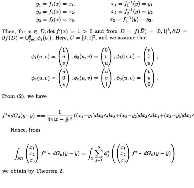
$D=[0,1]^{3}$

On

$D=[0,1]^{3}$,

we

consider the identity mapping

$y_{1}=f_{1}(x)=x_{1}$, $x_{1}=f_{1}^{-1}(y)=y_{1}$

$y_{2}=f_{2}(x)=x_{2}$, $x_{2}=f_{2}^{-1}(y)=y_{2}$

$y_{3}=f_{3}(x)=x_{3}$, $x_{3}=f_{3}^{-1}(y)=y_{3}$

.

Then, for $x\in D,$_{$\det f’(x)=1>0$} and from $D=f(\overline{D})=[0,1]^{3},$$\partial D=$ $\partial f(D)=\bigcup_{j=1}^{6}\phi_{j}(U)$. Here, $U=[0,1]^{2}$, and we

assume

that

$\phi_{1}(u, v)=(\begin{array}{l}1uv\end{array}),$ $\phi_{2}(u, v)=(\begin{array}{l}0vu\end{array}),$$\phi_{3}(u, v)=(\begin{array}{l}v1u\end{array})$ ,

$\phi_{4}(u, v)\vec{-}(\begin{array}{l}u0v\end{array}),$ $\phi_{5}(u, v)=(\begin{array}{l}uv1\end{array}),$$\phi_{6}(u, v)=(\begin{array}{l}vu0\end{array})$ .

From (2),

we

have

$f^{*}*dG_{3}(y- \overline{y})==\frac{1}{4\pi|x-\overline{y}|^{3}}((x_{1}-\overline{y}_{1})dx_{2}\wedge dx_{3}+(x_{2}-\overline{y}_{2})dx_{3}\wedge dx_{1}+(x_{3}-\overline{y}_{3})dx_{1}\wedge dx_{2})$

.

Hence, from

$/_{\partial D} (\begin{array}{l}x_{1}x_{2}x_{3}\end{array})f^{*}*dG_{n}(y-\overline{y})=\int_{U}\sum_{j=1}^{6}\phi_{j}^{*}((\begin{array}{l}x_{1}x_{2}x_{3}\end{array})f^{*}*dG_{n}(y-\overline{y}))$

(15)

$f^{-1}( \overline{y})=\frac{1}{4\pi}/_{0^{1}}/_{0^{1}}(\frac{1-\overline{y}_{1}}{|\phi_{1}-\overline{y}|^{3}}(\begin{array}{l}1uv\end{array})+\frac{\overline{y}_{1}}{|\phi_{2}-\overline{y}|^{3}}(\begin{array}{l}0vu\end{array})+\frac{1-\overline{y}_{2}}{|\phi_{3}-\overline{y}|^{3}}(\begin{array}{l}v1u\end{array})$

$+ \frac{\overline{y}_{2}}{|\phi_{4}-\overline{y}|^{3}}(\begin{array}{l}u0v\end{array})+\frac{1-\overline{y}_{3}}{|\phi_{5}-\overline{y}|^{3}}(\begin{array}{l}uv1\end{array})+\frac{\overline{y}3}{|\phi_{6}-\overline{y}|^{3}}(\begin{array}{l}vu0\end{array})$ $dudv$

$- \frac{1}{4\pi}\int_{0}^{1}\int_{0}^{1}\int_{0}^{1}\frac{1}{|x-\overline{y}|^{3}}(\begin{array}{l}x_{1}-\overline{y}_{1}x_{2}-\overline{y}_{2}x_{3}-\overline{y}_{3}\end{array})dx_{1}dx_{2}dx_{3}$

.

the graphs of $f^{-1}$ on $\{\overline{y}_{0}\in[0.1,0.9|^{3}|\overline{y}_{3}=0.5\}$.

Acknowledgements

S. Saitoh is supported in part by the Grant-in-Aid for Scientffic Research

(C)(2)(No. 19540164) from the Japan Society for the Promotion Science.

References

[1] S. Saitoh, Representations

_of

inverse functions, Proc. Amer. Math.

Soc., 125 (1997), 3633-3639.

[2] S. Saitoh, Integral Transforms, Reproducing Kemels and Their

Ap-plications, Pitman Res. Notes in Math. Series 369, Addison Wesley

Longman Ltd (1997), UK.

[3] Y. Sawano, M. Yamada and S. Saitoh, Singular integrals and natural

(16)

[4] M. Yamada, T. Matsuura and S. Saitoh, Representations

_of

inverse

functions

by the integral

_transform

with the sign kemel, Fract. Calc,

Appl. Anal., 10(2007), 161-168.

[5] M. Yamada and

S.

Saitoh,

_{Identifications of}

non-linear systems, J.

Comput. Math. Optim., 4(2008), 47-60.

[6] M. Yamada and S. Saitoh, 2-nonlinearsimultaneous equations, Appl,

Anal. (to appear).

Division of Electronics and Computing, Graduate School of Engineering,

Gunma University, Kiryu 376-8515, Japan,

Department ofMathematics, Graduate School of Engineering,

Gunma University, Kiryu 376-8515, Japan,

E-mail: [email protected],