Real algebraic links in $S^{3}$ and simple branched covers (Intelligence of Low-dimensional Topology)

全文

(1)13. Real algebraic links in S^{3} and simple branched covers Benjamin Bode Department of Mathematics, Osaka University. 1. Introduction. In contrast to the set of algebraic links, the real algebraic links in S^{3} are not classified yet. In this paper we aim to give an overview of work on this open problem. There are various instructive surveys on closely related topics such as Milnor fibrations and more general aspects regarding the topology of isolated critical points of polynomials [15, 17, 38, 39]. What this survey aims to add to the discussion is on the one hand an accessible treatment of the work that has already been done on the classification of real algebraic links without assuming any previous knowledge on the topic (apart from basic knot theory) and without any results that are not directly relevant for this question and might complicate the theory. This means that we are goin g to ignore otherwise very worthwile work on higher dimensions [3] and non‐isolated critical points [16, 19]. On the other hand we would like to point out connections to the theory of simple branched coverings of S^{3} over itself and the role of fibred links in this setting, in particular work by Montesinos and Morton [30]. This connection has not been spelled out explicitly before and we hope that it inspires future work on the cıassification of real algebraic links. The remainder of this paper is structured as follows. Section 2 gives the necessary definitions and background to state a conjecture by Benedetti and Shiota on the set of real algebraic links in S^{3} . Section 3 discusses the known constructions of real algebraic links, their similarities and limitations. In Section 4 we summarize results on branched coverings of S^{3} over itself and how these could lead to more general constructions. Acknowledgements: This work was supported by JSPS KAKENHI Grant Number JP18F18751 and a JSPS International Postdoctoral Fellowship. 2. Preliminaries. The central objects of this paper are polynomial maps whose vanishing sets contain knots and links in a very specific way. Before we give the definitions of algebraic and real algebraic links, we give the best‐known example due to Brauner [11]. Example: Consider the polynomial f : \mathbb{C}^{2}ar ow \mathbb{C} given by f(u,v)=u^{p}-v^{q} with p, q\in \mathbb{N}. More precisely, we are interested in its vanishing set on a 3‐sphere S_{p}^{3}=\{(u,v)\in \mathbb{C}^{2}:|u|^{2}+ |v|^{2}=p^{2}\} of a given radius p around the origin (0,0) \in \mathbb{C}^{2} . We can solve the polynomial equation or simply plot f^{-1}(0)\cap S_{\rho} for different values of p , but with either method we find. that it is T_{p,q} , the (p, q) ‐torus. hnk .. Remarkably, the link type does not depend on the radius. p.

(2) 14 at all. This is because the origin (0,0) is the only point (u,v)\in \mathbb{C}^{2} where f vanishes and where \nabla f(u,v)=\lambda(u,v) for some real \lambda . In this sense, the (p,q) ‐torus link is a very dominating feature of the vanishing set of f. We could now try to get rid of the property that the topology of f^{-1}(0)\cap S_{p}^{3} does not depend on p . We could simply multiply f by another complex polynomial g that does not vamish at the origin. Then for large \rho the link fg^{-1}(0)\cap S_{\rho}^{3} might be different from the (p,q) ‐torus link, but for small enough radii it is still T_{p,q} . The following definition captures the essential properties of f and fg. Definition 2.1. A link \bullet. L. is algebraic if there exists a polynomial f : \mathbb{C}^{2}ar ow \mathbb{C} such that. f has an isolated singularity at the origin, i. e., f((0,0))=0, \nabla f((0,0))=(0,0) and there. is a neighbourhood of \nabla f is notfull, \bullet. B. of (0,0)\in \mathbb{C}^{2} such that (0,0) is the only point in. f^{-1}(0)\cap S_{p}^{3}=L for all small enough radii. B. where the rank. p.. The polynomial u^{p}-v^{q} in the example has an isolated singularity at the origin. The fact that the singularity is isolated guarantees that the link type of the intersection f^{-1}(0)\cap S_{\rho}^{3} does not depend on p if it is small enough. Hence the (p,q) ‐torus link is algebraic. The algebraic links are compıetely classified and they tum out to be iterated cables of torus links, whose cabling coefficients satisfy an additional positivity condition. The precise result is not that important in this context. We recommend the excellent book by Eisenbud and Neumann [18] on the subject. For us it is for now enough to know that the algebraic links are classified and that they are a very small subset of the set of all links. The original construction of the polynomials in the example is due to Brauner [11], who also gave a description of all algebraic links in terms of their cabling coefficients. Work by Burau [12, 13, 14] then established that the links that one obtains from this description are actually distinct. The term ‘algebraic link’ is due to Lê [27]. Another excellent source for many interesting results in the theory of algebraic links is Milnor’s book [29], where he proves (among many other things) that if f has an isolated singularity at the origin, then the argument of f is a ıocally trivial fibration map over the circle, \arg f : S_{p}^{3}\backslash f^{-1}(0)arrow S^{1} for small enough. radii p.. Definition 2.2. A linkL is calledfibred if its complement S^{3}\backslash L is admits a locally trivialfibration over the circle S^{1} and the closures of the fibres are compact surfaces (Seifert surfaces) that intersect precisely in their common boundary L. Even if we didn’t know it from the classification of algebraic ıinks, we would now know from Milnor’s result that algebraic links are fibred. In the last chapter of his seminal work [29], Milnor investigates properties of the real ana‐ logue of links of isolated singularities of complex plane curves, which were later termed real algebraic links. We use this name in the sense of Perron [33] as links of isolated critical points of polynomials f : \mathbb{R}^{4}ar ow \mathbb{R}^{2} . This should not be confused with knotted algebraic varieties in \mathb {R}\mathb {P}^{3} as they were introduced by Viro [42], which are also called real algebraic links. Definition 2.3. A link. L. is real algebraic if there exists a polynomial f : \mathbb{R}^{4}ar ow \mathbb{R}^{2} such that.

(3) 15 \bullet. f has an isolated singularity at the origin, i. e., f((0,0,0,0))=(0,0), \nabla f((0,0,0,0))= and there is a neighbourhood B of the origin (0,0,0,0) such that (0,0,0,0) is the only point in B where the rank of \nabla f is notfull,. (\begin{ar ay}{l} 0 0 0 0 \end{ar ay}). \bullet. f^{-1}((0,0))\cap S_{p}^{3}=L for all small enough radii. p.. From now on we will usually write 0 for the origin in \mathb {R}^{4} , the origin in \mathb {R}^{2} and a matrix whose entries are all equal to zero. It should be clear from the context which of these we are referring to. In the literature one often also encounters the term “isolated critical point”. In this scenario the two terms can be used interchangeably. A critical point is a point, where the gradient does not have full rank, while a singularity refers to a point where the gradient is the matrix with 0 ‐entries. Via a change of coordinates, any critical point can be turned into a singularity. In Definition 2.3 the origin is a singularity, but is isolated in the sense of a critical point (it is the only point in a neighbourhood where the gradient does not have full rank). Definition 2.3 differs from Definition 2.1 only in that we replaced every instance of \mathb {C} by \mathb {R}^{2} . This might seem like a small change, but note that it enlargens the set of polynomials considerably. While every complex polynomial from Definition 2.1 can be written as a real polynomial as in Definition 2.3 by considering its real and imaginary parts, the converse is not true. It should be obvious that most real polynomials are not holomorphic for example. Hence, every algebraic link is real algebraic, but not vice versa. At first (around the time of Milnor’s book), it was not clear at all if there were any real algebraic links that are not algebraic, but even though the real algebraic links are not classified yet, we now have plenty of examples for this (cf. Section 3).. Both Definition 2.1 and Definition 2.3 can be generalized to higher dimensions and many of the results (such as Milnor’s fibration theorem) remain true.. One difference between the complex and the real polynomials is that in general the argument of a real polynomial as in Definition 2.3 (\arg f:S_{\rho}^{3}arrow S^{1}) is not a fibration. However, Milnor established that the following is still true. Theorem 2.4 (Milnor [29]). If a link. L. is real algebraic, then. L. is fibred.. According to Benedetti and Shiota this implication should be an equivalence. Conjecture 2.5 (Benedetti‐Shiota [5]). A link. L. is real algebraic if and only if. L. is fibred.. Akbulut and King showed that every link can be constructed around a weakly isolated singu‐ larity [2] meaning that the origin is allowed to lie on a component of the critical set of positive dimension as long as the origin is the onıy point in a neighbourhood where the critical set intersects the vanishing set f^{-1}(0) . The idea of Benedetti and Shiota is based on a procedure of blow‐ups and blow‐downs start‐ ing from a polynomial f with the properties from Akbulut and King. At this point however, an appropriate blow‐down technique is not made precise yet and Conjecture 2.5 remains conjec‐ tural.. Another result that might be interpreted as encouraging regarding Conjecture 2.5 is due to Kauffman and Neumann [26]. They showed that if you allow real analytic functions with so called tame singularities rather than only polynomials, then the links around these singularities are precisely the fibred links..

(4) 16 It should also be noted that real polynomial maps \mathbb{R}^{4}ar ow \mathbb{R}^{2} with isolated s i n gularities are rare, in the sense that a ‘generic’ polynomial map between these spaces has a critical set of dimension 1.. 3. Constructions of real algebraic links. In this section we review the different constructions of real algebraic links that have been de‐ veloped over the years. If this list is incomplete, it is only due to the author’s own limitations. At the moment the set of links that are known to be real algebraic is still comparatively small. There are of course the algebraic ıinks, but until Looijenga showed that the connected sum K#K of any fibred knot K with itself is real algebraic [28], it was not known if there would be any other examples. Looijenga in fact proved that every fibred knot K that is odd, i.e. can be realized as an invariant set under the inversion i,. i:S^{3}arrow S^{3}, i((u,v))=(-u, -v). such that the. fibration map is equivariant under is real algebraic. The basic idea of his construction is as follows. Use the fibration to define a map from a neighbourhood U of S^{3} to \mathbb{R}^{2}\cong \mathbb{C} , which vanishes on K and whose argument on S^{3} is equal to the fibration map. We can approximate this map by a polynomial map \Phi=(\Phi_{1},\Phi_{2}) : Uarrow \mathb {R}^{2} up to their first derivatives, which because of the symmetry of the fibration we can con‐ struct such that it consists only of terms with odd degrees. Therefore the rescaled function f=(f_{1},f_{2}) : \mathbb{R}^{4}ar ow \mathbb{R}^{2}, f_{i}(x)=\Phi(x/|x|)|x|^{\deg\Phi_{i}} is a polynomial. By construction this map satisfies the conditions from Definition 2.3. The singularity at the origin is isolated essentially because the fibration map does not have any critical points. Pichon showed that if f,g:\mathbb{C}^{2}arrow \mathbb{C} are holomorphic maps, then the function f\overline{g} has an isolated singularity at the origin if and only if L_{f\overline{g} :=f\overline{g}^{-1}(0)\cap S_{\varepsilon}^{3} is a fibred link [34]. Note that the link of this singularity f\overline{g}\cap S_{\varepsilon}^{3} is the umion of L_{f}=f^{-1}(0)\cap S_{\varepsilon}^{3} and the L_{\overline{g}}=L_{g} := g^{-1}(0)\cap S_{\varepsilon}^{3} . In particular, if f and g are complex polynomials, then L_{f} and L_{g} are algebraic links. That in general the resulting link L_{\int\overline{g} is not algebraic, can be seen for example from [25]. Functions of the form f\overline{g} with holomorphic polynomials f and g have taken a prominent role in the construction of isolated critical points since A’Campo’s first example in this context [1]. Perron [33] and Rudolph [36] independently constructed polynomials for the figure‐eight knot 4_{1} , which is neither odd nor algebraic. This construction is also based on a particularly symmetric parametrisation. Perron considers a parametrisation of a braid that closes to 4_{1} in terms of trigonometric functions. This leads him to a parametrisation of 4_{1} itself in a 3‐sphere of a given radius and consequentially to a polynomial (f_{1},f_{2}):\mathbb{R}^{4}arrow \mathbb{R}^{2} whose nodal set on that 3‐sphere is 4_{1} . The elegance of this lies in the simplicity of the resulting polynomial. It requires only 6 terms in total and is of degree 3, while the polynomials in Looijenga’s construction for example can have arbitrarily large degree. Furthermore and like in Looijenga’s construction, the symmetries of the original braid parametrisation mean that all terms of (f_{1},f_{2}) have odd degree. The polynomial map with an isolated singularity is then obtained (exactly like in Looijenga’s construction) by considering the radially rescaled function |x|^{3}(f_{1}(x/|x|),f_{2}(x/|x|)) . Showing that the singularity at the origin is indeed isolated requires some tedious calculations. In this regard, Rudolph’s construction is more satisfying as his functions can be written as a polynomial in complex variables u, v and the complex conjugate \overline{v} , which makes the proof of the isolated singularity significantly easier..

(5) 17 Perron’s construction can be generalized to a much larger class of braids as we pointed out in [9]. s-1. Definition 3.1. A braid B on s strands is called homogeneous iffor every i=1,2, generator \sigma_{i} appears in the word B if and only if \sigma_{i}^{-1} does not appear.. the. We showed in [9] that all closures of squares of homogeneous braids are real algebraic. Like in Perron’s construction we start with a braid parametrisation that involves trigonometric functions. Let B be a homogeneous braid and let s_{C} be the number of strands that form the component C of the closure of B . Hence the number of strands s of B equals \sum_{C}s_{C} . We require parametrisations of the form. \bigcup_{Cj}\bigcup_{=1}^{sc}(F_{C}(\frac{t+2\pi j}{s_{C} ), G_{C}(\frac{t+ 2\pi j}{s_{C} ),t) , t\in[0,2\pi]. ,. (1). where F_{C}, G_{C}:[0,2\pi]arrow \mathbb{R} are trigonometric polynomials. We then define g_{\lambda} : \mathbb{C}\cross S^{1}arrow \mathbb{C}.. g_{\lambda}(u,t)= \prod_{Cj}\prod_{=1}^{s_{C} (u-\lambda(F_{C}(\frac{t+2\pi j} {s_{C} )+iG_{C}(\frac{t+2\pi j}{s_{C} ) ). ,. (2). which has the closure of B in \mathbb{C}\cross S^{1} as its vanishing set for all \lambda>0 . We show in [8] that we can find for every homogeneous braid a parametrisation as in Eq. (1) such that \arg g_{\lambda} :. ( \mathbb{C}\cross Sı) \backslah g‐ (0)arrow S^{1} is a fibration map.. Note that the fibration property of \arg g_{\lambda} can be phrased entirely in terms of the critical values of g_{\lambda} . For a fixed value of t the criticaı values of g_{\lambda}(u,t) are given by v_{i}(t)=g_{\lambda}(c_{i},t) with s-1 . Then \arg g_{\lambda} is a fibration if and onıy if for all i the derivative =0, i=l,2 ,. \frac{ \partilg_{\ambd}{\partil \partilu}(c_{igv}(t) {\partilvanishest) } never . This has a nice geometric interpretation in terms of the movements. of the critical values in the complex plane as t varies. Note that they are always non‐zero and the non‐vanishing derivatives of their arguments mean that they never change the orientation in which they twist around 0 as t varies between 0 and 2\pi . For every v_{i}(t) this twisting is either always clockwise. ( \frac{\partial\arg v_{i}(t)}{\partial t}<0) or always anti‐clockwise ( \frac{\partial\arg v_{i}(t)}{\partial t}>0) . (v_{i}(t),t)\subset \mathbb{C}\cross[0,2\pi] s=\deg(g_{\lambda}) strands. It turns. The union of the critical values. \mathbb{C}\cross[0,2\pi]. form a braid A on. of. g_{\lambda}(u,t). (0,t)\subset g_{\lambda}(u,t) such. and the curve. out that we can take. that there is a close relation between this braid and the braid B that is formed by the roots of , then A can be taken to be a conjugate of g_{\lambda}(u,t) . Namely, if we write. B= \prod_{j=1}^{\el }\sigma_{i_{j} ^{\varepsilon_{j}. where. A=\prod_{j=1}^{\el}A_{i j}^{\varepsilon_{j}. ,. (3). X_{i}=\sigma_{i}^{-1}\sigma_{i-1}^{-1}\ldots\sigma_{2}^{-1}\sigma_{1}^{2} \sigma_{2}\ldots\sigma_{i-1}\sigma_{2},. A_{i}=\{ begin{ar y}{l X_{\frac{i+1}{2} if sod , X_{\frac{i}2+\lfo r\fac{s}2\rflo r} if sev n. \end{ar y}. (4).

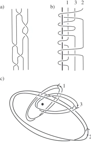
(6) 18 This is shown in [9] and stems from an idea in [37]. Note that if can be parametrised such that. \frac{\partial\arg v_{i}(t)}{\partial t} never vanishes.. B. is homogeneous, then. A. The example of the homogeneous braid. B=\sigma_{1}\sigma_{2}\sigma_{1}\sigma_{3}^{-2}\sigma_{2} is illustrated in Figure 1. In the context of Section 4 it is an important observation that not only does the union of the critical values. on. s. (v_{i}(t),t)\subset \mathbb{C}\cross[0,2\pi] of g_{\lambda}(u,t) and the curve (0,t)\subset \mathbb{C}\cross[0,2\pi] form a braid (0,t) is a braid axis for the union of the critical values (v_{i}(t),t)\subset \mathbb{C}\cross S^{1}.. strands, but also. The closure of this braid is an. s-1 ‐component. unlink.. When we expand the product in Eq. (2) we obtain a polynomial in the complex variable u , but also in e^{it} and e^{-it}.. The function g_{\lambda}(u,2t) then also gives a fibration map via its argument and has the closure of B^{2} as its vanishing set. Furthermore, expanding the product results in a polynomial in u, e^{\dot{ \imath} t} and e^{-it} , where all exponents of e^{it} and e^{-it} are even. We define a real polynomial in \mathbb{C}^{2}\cong \mathbb{R}^{4}ar ow \mathbb{R}^{2}\cong \mathbb{C} by rescaling g_{\lambda} :. f_{\lambda}(u,v)=\{ begin{ar ay}{l} r^{2k\Sigma_{C}s_{C}g_{\lambda}(\frac{u}{r^{2k},2t), ifv=re^{\dot{\imath} }t u^{s} ifv=0, \end{ar ay}. (5). with k \geq\max\{\deg_{e^{it}}g_{\lambda},\deg_{e} ıt g_{\lambda}\}/2s . Then f_{\lambda} can be written as a polynomial in u, v and \overline{v}. This is because the exponents of and in g_{\lambda} are even and therefore cancel. e^{it}=\frac{v}{\sqrt{v\overline{v}. e^{-\dot{ \imath} t =\frac{\overline{v} {\sqrt{v\overline{v}. the square roots. Moreover, f_{\lambda} has an isolated singularity at the origin and if \lambda is small enough, the link around that singularity is the closure of B^{2} by construction. The details of these constructions go beyond the scope of this short overview. What we would like to highlight are the striking similarities between the different constructions. All of them (apart from the ones based directly on algebraic links such as Pichon’s [34]) start with a particular parametrisation of the desired knot or link L. Usming this parametrisation we then define a function whose vanishing set is in some sense L (either on a 3‐sphere or on \mathbb{C}\cross S^{1} ) and then perform some sort of rescaling argument to obtain the desired polynomial (eliminating. |x|=\sqrt{x_{1}^{2}+x_{2}^{2}+x_{3}^{2}+x_{4}^{2} |v|=\sqrt{x_{3}^{3}+x_{4}^{2}. the dependence on either the modulus or ). There are two main obstacles to look out for. Firstly, rescaıing, whether radially or by the modulus of v, introduces square root terms. We can therefore in general not expect to obtain a polynomial. This is only achieved if the parametrisation we started with has some particular symmetries. In the case of Looijenga’s construction, this means that we have to limit ourselves to odd knots. In the construction in [9], it requires us to only consider closures of 2‐periodic braids. It is not a coincidence at all that both of these symmetries are related to the number 2, the exponent that cancels a square‐root term. The second obstacle is that we need to make sure that we have an isoıated singularity. In the previous constructions this is closely linked to explicit fibration maps over the circle. Looi‐ jenga’s construction starts with the fibration, so it is clear that we need a fibred link to start with. Having Milnor’s theorem in mind this turns out not to be a restriction at all. In [9] we have to limit ourselves to homogeneous braids because these are the ones, for which we know how to construct polynomial fibrations that are holomorphic in u. In both our [9] and Rudolph’s construction the resulting polynomial is semiholomorphic: It can be written as a polynomial in complex variables u, v and \overline{v} . This makes it a lot easier to.

(7) 19. a). b). 1 3 2. c). Figure 1: A simple relation between the braid that is formed by the critical values of a loop in the space of polynomials and the braid that is formed by the roots of the same polynomials. a) The braid B=\sigma_{1}\sigma_{2}\sigma_{1}\sigma_{3}^{-2}\sigma_{2}. b) B can be parametrised such that it is given by the roots of a loop in the space of complex polynomials, whose critical values and the 0 ‐strand. (0,t)\subset \mathbb{C}\cross[0,2\pi]. form the braid. A=A_{1}A_{2}A_{1}A_{3}^{2}A_{2}=X_{1}X_{3}X_{1}X_{2}^{2}X_{3} .. The number. above a strand gives a correspondence between the Artin generator \sigma_{i} and one twist of that strand around the 0‐ strand. c) The top view of the braid in b). The critical values (i.e., A without the 0 ‐strand) can be parametrised such that \frac{\partial\arg v_{i}(t)}{\partial t} never vanishes. They form a s-1 ‐component unlink and the 0 ‐strand is a braid axis for it. i.

(8) 20 check that the singularity is isolated. Semiholomorphic polynomials are special cases of mixed polynomials that are studied in the context of singularities in [32, 35, 38]. In lack of a better term we call a link semiholomorphic if it is the link of an isolated singularity of a semiholomorphic polynomial \mathbb{R}^{4}ar ow \mathbb{R}^{2} . It is a natural question to ask if the set of semiholomorphic links is the same as the set of real algebraic links. Theorem 3.2 (Looijenga [28], Perron [33], Pichon [34], Rudolph [36], Bode [9]). The links that are known to be real algebraic are as follows: \bullet. \bullet. algebraic links,. L_{f\overline{g} , the link of the singularity of f\overline{g}, where f and isolated singularities, i.e. L_{f}\sqcup L_{g} if it is fibred. g. are holomorphic polynomials with. \bullet. oddfibred links (including K#K for. \bullet. the closure of B^{2} if B is a homogeneous braid (including 4_{1} ).. K. a fibred knot),. Out of these, the algebraic links and closures of squares of homogeneous braids are known to be semiholomorphic as well.. Recently, the techniques from [9] have been further generalised to constructions of families of links that might not be closures of homogeneous braids [10]. The underlying principle of symmetric parametrisations and rescaling remains the same though. It remains challenging to check whether the newly constructed links in [10] are already known to be real algebraic from Theorem 3.2.. Branched coverings of S^{3} over itself and Hopf plumbings. 4. So far, all proofs of real algebraicity of links are constructive and all constructions are either based on aıgebraic links (as in Pichon’s construction) or on a rescaling of a polynomial, whose vamishing set on a subset of \mathb {R}^{4} is the desired link. This rescaling introduces square root terms and naturally restricts the class of links for which the resulting function is a polynomial to those that satisfy certain symmetry constraints. This not only means that it is doubtful that this approach can prove the conjecture by Benedetti and Shiota, but also makes it very hard to check if a link falls into that class as it might not be straightforward to investigate if it possesses the necessary symmetries. A proof of the conjecture of Benedetti and Shiota should therefore not involve an exact radial rescaling. In Looijenga’s construction for example, the argument map S_{p}^{3}\backslash Larrow S^{1} given by the. p=|x|=\sqrt{x_{1}^{2}+x_{2}^{2}+x_{3}^{2}+x_{4}^{2} . In the construction in [9] the argument of f_{\lambda}(u, re^{it}) does not depend on r=|v|=\sqrt{x_{3}^{2}+x_{4}^{2} . Instead argument of the polynomial does not depend on the radius. it is probably worth looking for a way to construct a polynomial map f : \mathbb{R}^{4}ar ow \mathbb{R}^{2} with an roma nther or ingu1 \arg fdoesd S^{3}\backslash Larrow S^{1},. hatitisverysma11;sma11enoughiso1 \frac{\partialargn\chi_{f} {u1ar\partial\rho}=0wecou1d e.. ythe nsurmatedse t arInitstyonstefadoructeavifdsibrnagtio : atwhered mOeandtourse, ependoonsideratiadionsausp odu1usr.. toe. hatthec. fh. ingityissti11iso1. fc. simi1arc. pp1.

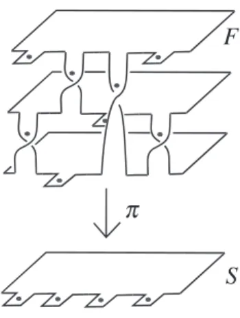
(9) 21 21. \Downar ow\pi Figure 2: A 3‐sheeted simple branched cover of a disc. The branch set Q consists of 4 points.. to the dependence on r . This is all very vague at the moment and it is not clear at all how such a construction could be achieved.. If such a rescaling could be defined, it would be easier to check whether the resulting function has an isolated singularity if it is a semiholomorphic polynomial. Hence, while we still lack a proper rescaling mechanism, we can investigate for which fibred links the fibration map can be taken to be the argument of a semiholomorphic polynomial. From [8] we know this for closures of homogeneous braids, but recently there have been constructions of links that appear not to be homogeneous braid closures [10]. It would obviously be desirable if the construction of isolated singularities (or the construc‐ tion of semiholomorphic polynomial fibrations) did not start with some particular parametri‐ sation or symmetry requirement, but rather with a property that is satisfied by all fibred links. While there are several at hand, for some of them, such as properties of the commutator sub‐ group of the link group [40] or knot Floer homology [31], it might not be easy to establish a connection to the topic of polynomial maps. There are however two properties where such a connection might exist, the first being the study of branched coverings of S^{3} over itself. The following exposition foılows Montesinos and Morton [30]. Definition 4.1. Let \pi. F. and. S. be surfaces and let. is a simple branched cover with. d. \pi:Farrow S. be a continuous surjective map. Then. sheets if there is a finite branch set Q\subset int(S), where int(S). denotes the interior of S, such that.‘ \bullet. \bullet. \pi|_{F\backslash \pi^{-1}(Q)}. is a d ‐sheeted covering map,. for every q\in Q there is a neighbourhood U such that \pi^{-1}(U) has d-1 components, one of which is a disc that is projecting to U as a double cover branched over q, while the others are discs that are projecting homeomorphically.. The concept of a simple branched cover is illustrated in Figure 2..

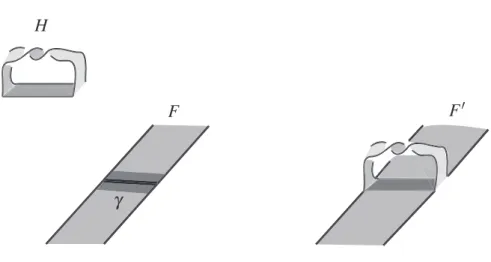
(10) 22 Definition 4.2. Let M and N be closed 3‐manifolds. A map \pi : Marrow N is called a simple d‐ sheeted cover with branch set C\subset N if it is locally homeomorphic to the product of an interval with a simple d ‐sheeted cover of a disc, and the branch points in the productform the set C. Now let L_{branch} be a link in. S^{3}. and O be an unknot in. S^{3}. such that O is a braid axis for. L_{branch} , i.e., there is a fibration of S^{3}\backslash O over the circle such that each fibre surface intersects L_{branch} the same number of times and the intersections are transverse. Let \pi : S^{3}arrow S^{3} be a simple branched cover of S^{3} over itself, with branching set L_{branch} . Then \pi^{-1}(O) is a fibred link in S^{3} and conversely, for every fibred link there are such links L_{branch} , braid axes O and covers \pi . The relation between fibred links and simple branched covers has been studied extensively by Birman [6], Goldsmith [22], Hilden [24] and Montesinos with Morton [30]. This relates to the construction of semihoıomorphic fibrations as follows. Consider a semiholomorphic polynomial f : \mathbb{C}^{2}ar ow \mathbb{C} constructed as in [9]. In particular, \arg f : (\mathbb{C}\cross rS^{1})\backslash f^{-1}(0)arrow S^{1} is a fibration for all r>0 . Since \arg f(u, re^{it}) goes to \arg u^{s} and |f(u, re^{it})| goes to infinity for all re^{it} as |u| goes to infinity, we can compactify \mathbb{C}\cross S^{1} to S^{3}. This way the map. ( \frac{u}{1+|u|},e^{it})\mapsto(\frac{f(u,re^{it})}{1+|f(u,re^{it})|},e^{it}). ,. (e^{i\chi},0)\mapsto(e^{is\chi},0). (6). is a branched covering of S^{3} over itself for every value of r . Here we have identified S^{3} with. (\mathbb{D}\cross S^{1}). modulo. (e^{\dot{ \imath} \chi},e^{\dot{ \imath} t_{1} )=(e^{\dot{ \imath} \chi},e^{it_ {2} ). for all \chi, t_{1} , t_{2} , where \mathb {D} is the cıosed unit disc in \mathbb{C}.. The maps in (6) are branched over the set. ( \frac{v_{i}(t)}{1+|v_{i}(t)|},re^{it})=(\frac{f(u,re^{it})}{1+|f(u,re^{\dot{ \imath} t})|},e^{it}) s-1 ,. where i=1,2,. \frac{\partial f}{\partial u}(u, re^{it})=0 .. ,. (7). Recall from the remark in Section 3 that this set is. \frac{0\arg v_{i}(t)}{\partial t}. s-1 ‐component. a unlink and that \arg f being a fibration implies that the derivative never vamishes. This implies that (0,e^{it}) is a braid axis for \bigcup_{i}(v_{i}(t)/(1+|v_{i}(t)|),e^{it}) . Since. f^{-1}(0)\cap(\mathbb{C}\cross rS^{1}). is the constructed fibred link. L,. the functions that are constructed in [9] can. be explained in the context of [30]. There is a second obvious braid axis for \bigcup_{i}(v_{i}(t)/(1+|v_{i}(t)|),e^{it}) , namely (e^{i\chi},0) , \chi\in [0,2\pi] , and its preimage under branched covering map is the unknot (e^{i\chi},0) , \chi=[0,2\pi]. Therefore every semiholomorphic link L that is constructed as in [9] gives rise to a simple s ‐sheeted cover \pi:S^{3}arrow S^{3} with branch set L_{branch} , which is an s-1 ‐component unlink, such that. L=\pi^{-1}(O). for some braid axis O for L_{branch} . Furthermore, there is another braid axis O'. for L_{branch} whose preimage set under \pi is an unknot. In fact, O' is a braid axis for O\cup L_{branch} and O\cup L_{branch} is an s ‐strand braid with respect to O'. We will revisit this idea once we have introduced the second property of fibred links that could be useful in the context of polynomial singularities. We call an unknotted annulus with a positive or negative full twist a positive or negative. Hopf band. Let. F. be a fibre surface and. \gamma. an arc, i.e., a simple path in int (F) except for its. endpoints, which lie in \partial F . A neighbourhood. U. of \gamma in. F. is then a properly embedded square.

(11) 23 H. F'. F. Figure 3: A Hopf band. H. is plumbed to a surface. F. along a path \gamma.. which has two opposite sides in \partial F . Similarly, we consider a square U'\subset H with two opposite sides on \partial H . A Hopf pıumbing along \gamma is obtained from F by glueing H to F by identifying U and U' such that the two sides of U' in \partial H run parallel to \gamma. We also say a surface F' is obtained from F by deplumbing a (positive or negative) Hopf band if F is obtained from F' by Hopf plumbing. Analogously, we say a fibred link L'=\partial F' is obtained from L=\partial F by Hopf plumbming if the corresponding fibre surface F' is obtained from F by Hopf plumbing. An illustration of Hopf plumbing is shown in Figure 3. If L is a fibred link, then so are aıl links that are obtained from it by Hopf plumbing and deplumbin g[20,41] . Conversely, Giroux and Goodman showed the following theorem, which was originally conjectured by Harer [23]. Theorem 4.3 (Giroux‐Goodman [21]). Every fibred link can be obtained from the unknot through a sequence ofHopfplumbings and deplumbings.. Montesinos and Morton established a connection between these two concepts, branched cov‐ erings of S^{3} over itself and Hopf plumbings, and thereby also a connection between sequences of Hopf plumbings and polynomial fibrations. At the time of their work, Harer’s conjecture was still unproven and it is not far‐fetched to believe that they hoped to make progress on Harer’s conjecture using their idea of branched coverings. Let \pi:S^{3}arrow S^{3} be simple branched covering with branch set L_{branch} . Let O be a braid axis for L_{branch} and \phi : S^{3}\backslash Oarrow S^{1} be a fibration such that each fibre intersects L_{branch} transversally in precisely s-1 points. Let D be a fibre of \phi and \gamma be a simple path in D starting at one of the points in D\cap L_{branch} , ending at the boundary \partial D and avoiding all points in D\cap L_{branch} in between. Let U be an open neighbourhood of \gamma in S^{3} . Now we push D\cap U in the normal direction of D and connect this push‐off with \partial D . This means we have attached a disc to D that in some sense ıies directly over the path \gamma. Near the starting point of \gamma which is in D\cap L_{branch}, this disc intersects L_{branch} . We apply a positive or negative half‐twist to the attached disc before this intersection. The result should look similar to Figure 4..

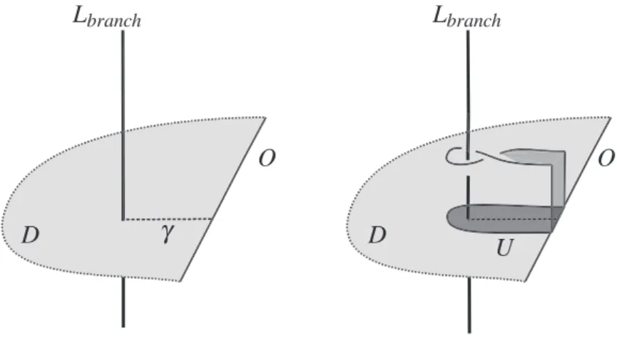
(12) 24 Lbranch. Lbranch. ... ... :: :. D. ::=D =. Figure 4: The dotted line is a path \gamma from the intersection of L_{branch} with D to O=\partial D . A neighbourhood U of that path is pushed off D . Applying a half‐twist to this pushed‐off disc results in this figure. The disc D' is the union of D and the pushed‐off disc with a half‐twist.. Note that by attaching this twisted disc to. D. we have constructed a new disc D' that intersects. L_{branch} in s points, one more than D . Furthermore, the boundary of D' is also a braid axis for L_{branch} . The braid word of L_{branch} with respect to \partial D' can be obtained from the braid with. respect to \partial D by a conjugation that depends on the path \gamma and Markov stabilization \sigma_{s-1}^{\pm 1} , where the sign depends on the sign of the half‐twist of the attached disc. Since \partial D' is a braid axis for L_{branch} , its preimage under the same covering map \pi is a fibred link L' just like L=\pi^{-1}(\partial D) is fibred.. Theorem 4.4 (Montesinos‐Morton [30]). Let the situation be as described above. Let F= \pi^{-1}(D) be the fibre surface of L. Then there is a path \tilde{\gam a} in F , starting and ending at \partial F with \pi(\tilde{\gamma})=\gamma such that F'=\pi^{-1}(D') , the fibre surface of L' , is up to isotopy obtained from F by Hopfplumbing along \tilde{\gam ,a} where the sign of the Hopfplumbing depends on the sign of the half‐ twist in the attached disc or equivalently the sign of the Markov stabilization that converts the braid word of L_{branch} with respect to \partial D into the braid word of L_{branch} with respect to \partial D'.. Corollary 4.5 (Montesinos‐Morton [30]). If O and O' are braid axes for the same link L_{branch} in S^{3} , which is the branch set of a simple branched covering \pi : S^{3}arrow S^{3} , then \pi ‐ı(O) and. \pi^{-1}(O'). are related by a sequence of Hopfplumbings and deplumbings.. This corollary is nowadays obvious because Giroux’s and Goodman’s work tells us that all fibred links are related by such sequences. The remarkable insight is the close connecting between Hopf plumbings and changes of the braid axis. It is also important to note that the converse of Theorem 4.4 and Corollary 4.5 is not known. It is not clear if we can always arrange that the path along which the plumbing or deplumbing happens can be arranged to lie over \gamma as in the Theorem. If a Hopf plumbing (or deplumbing) can be obtained as above, then we say that it corresponds to a Markov move. Montesinos and Morton raised the followin g question..

(13) 25 Question 4.6 (Montesinos‐Morton [30]). Can every fibred link be obtained as the preimage of a braid axis of an s-1 ‐component unlink L_{branch} under a simple s ‐sheeted branched covering \pi:S^{3}arrow S^{3} , whose branch set is L_{branch^{7}}. By the earlier remark this would imply that every fibred link can be obtained from the unknot via a sequence of Hopf plumbings and deplumbings, all of which correspond to Markov moves on the branch set of the branched covering \pi . At the time a positive answer to this question would have been the first proof of Harer’s conjecture. However, even now that Harer’s conjec‐ ture is proven, it is still not known if this question by Montesinos and Morton has a positive answer.. For the construction of more real algebraic links we would like to go beyond Montesinos and Morton’s question. Question 4.7. Can every fibred link L be obtained as a the preimage of a braid axis O of an s-1 ‐component unlink L_{branch} under a simple s ‐sheeted branched covering \pi:S^{3}arrow S^{3} , whose branch set is L_{branch} and the braid index of O\cup L_{branch} is s^{7} The braid index of O\cup L_{branch} being equal to s is equivalent to sayin g that there is a braid axis O' for O\cup L_{branch} with \pi^{-1}(O') being an unknot. Note that this question can just like Montesinos and Morton’s question be interpreted as a question on whether it is possible for every link to find a sequence of Hopf plumbings and deplumbings that has certain additional properties. Recall that the situation described in this question is precisely what we encounter for the simple branched covering from a semiholomorphic link as in [9]. Suppose that the answer to the question above is positive. Then maybe there is a way to construct from the simple branched coverin g\pi a polynomial map g_{\lambda} : \mathbb{C}\cross S^{1}arrow \mathbb{C} , whose argument is a fibration. Whether or not this is possible depends on the answer to the following question. Question 4.8. Let X_{s} denote the space of simple s ‐sheeted branched covers of the disc \mathbb{D} over itself such that 0\in \mathbb{D} is not in the branch set. Is every loop in X_{s} homotopic to a loop in the space V_{s} of complex polynomials of degree s with distinct non‐zero critical values? Note that V_{s} is a subset of X_{s} and usin g results from [4] and [7] a positive answer would imply that for every fibred link there is a semiholomorphic polynomial f : \mathbb{C}^{2}ar ow \mathbb{C} such that. f^{-1}(0)\cap S^{3}=L (and f^{-1}(0)\cap(\mathbb{C}\cross S^{1})=L ) and \arg f|_{S^{3}\backslash L} is a fibration.. Subject to an appropriate rescaling mechanism that does not rely on particular symmetries to yield polynomials (which admittedly comes with its own problems and difficulties), this could result in a construction of polynomial isolated singularities for any fibred link and hence in a proof of the conjecture by Benedetti and Shiota. At the moment this is still highly speculative, but we hope that this exposition inspires future work on the classification of real algebraic links. References. [1] N. A’Campo. Le nombre de Lefschetz d’une monodromie. Indag. Math. 35 (1973), 113‐ 118..

(14) 26 [2] S. Akbulut and H. King. All knots are algebraic. Commentarii Mathematici Helvetici 56, 1 (1981), 339‐351.. [3] R. N. Araújo dos Santos, M. A. B. Hohlenwerger, O. Saeki and T. O. Souza. New examples ofNeuwirth‐Stallings pairs and non‐trivial Milnorfibrations. Annales de l’Institut Fourier 66 (2016), 83‐104.. [4] A. F. Beardon, T. K. Carne and T. W. Ng. The critical values of a polynomial. Constr. Approx. 18 (2002), 343‐354. [5] R. Benedetti and M. Shiota. On real algebraic links on S^{3} . Bolletino dell’Unione Mathe‐ matica Itahana, Serie 8 Volume 1B. 3 (1998), 585‐609.. [6] J. S. Birman. A representation theorem for fibered knots and their monodromy maps. Topology of low‐dimensional manifolds. Lecture Notes in Mathematics 722 (Springer, Berlin), R. Fenn (ed.) (1977), 1‐8.. [7] B. Bode, M. R. Dennis, D. Foster and R.P. King. Knotted fields and explicit fibrations for lemniscate knots. Proc. R. Soc. A 473 (2017), 20160829.. [8] B. Bode and M. R. Dennis. Constructing a polynomial whose nodal set is any prescribed knot or link. Journal of Knot Theory and its Ramifications 28, no. 1 (2019), 1850082. [9] B. Bode. Constructing links of isolated singularities of real polynomials \mathbb{R}^{4}ar ow \mathbb{R}^{2} . Journal of Knot Theory and its Ramifications 28, no. 1 (2019), 1950009. [10] B. Bode. Braid group actions on the n ‐adic integers. arXiv:1903.06308 (2019). [11] K. Brauner. Zur Geometrie der Funktionen zweier komplexen Veränderlichen Il, IlI, lV. Abh. Math. Sem. Hamburg 6 (1928), 8‐54.. [12] K. Burau. Kennzeichnung von Schlauchknoten. Abh. Math. Sem. Hamburg 9 (1933), 125‐ 133.. [13] K. Burau. Kennzeichnung von Schlauchverkettungen. Abh. Math. Sem. Hamburg 10 (1934), 285‐297.. [14] W. Burau. Über Zopfgruppen und gleichsinnig verdrillte Verkettungen. Abh. Math. Sem. Hamburg 11 (1936), 179‐186.. [15] N. Dutertre. Topology of real singularities. In: Singularities and Foliations. Geometry, Topology and Applications. R. N. Araujo dos Sontas, A. Menegon Neto, D. Mond, M. J. Saia, J. Snoussi (Eds.), Sprminger International Publishing. (2018), 51‐88. [16] N. Dutertre and R. N. Araújo dos Santos. Topology of real Milnor fibrations for non‐ isolated singularities. Intemational Mathematics Research Notices 2016 (2016), 4849‐ 4866.. [17] N. Dutertre, R. N. Araújo dos Santos, Y. Chen and A. Andrade. Fibrations structure and degree formulae for Milnorfibers. arXiv: 1409.5053 (2014)..

(15) 27 [18] D. Eisenbud and W. Neumann. Three‐dimensional link theory and invariants of plane curve singularities. Princeton University Press (1985). [19] J. Fernández de Bobadilla and A. Menegon Neto. The boundary of the Milnor fibre of complex and real analytic non‐isolated singularities. Geometriae Dedicata 173 (2014), 143‐162.. [20] D. Gabai. Detecting fibred links in S^{3} . Comm. Math. Helvetici 61 (1986), no. 1, 519−555 [21] E. Giroux and N. Goodman. On the stable equivalence of open books in three‐manifolds. Geometry & Topology 10 (2006), 97‐114.. [22] D. Goldsmith. Symmetric fibered links. Knots, groups and 3‐manifolds, Annals of Mathe‐ matics Studies 84, Princeton University Press (1975), 3‐23.. [23] J. Harer. How to construct all fibered knots and links. Topology 21, 3 (1982), 263‐280. [24] H. M. Hilden. Three‐fold branched coverings of S^{3} . Amer. J. Math. 98 (1976), 989‐997. [25] M. Ishikawa. On the contact structre of a class of real analytic germs of the form f\overline{g}. Advanced Studies in Pure Mathematics 56 (2009), Singuıarities—Nigata‐Toyama 2007, 201−223.. [26] L. H. Kauffman and W. D. Neumann. Products of knots, branched fibrations and sums of singularities. Topology 16 (1977), 369‐393. [27] D. T. Lê. La monodromie n ’a pas de points fixes. J. Fac. Sci. Univ. Tokyo Sect. IA Math. 22 no. 3 (1975), 409‐427.. [28] E. Looijenga. A note on polynomial isolated singularities. Ind. Math. (Proc.) 74 (1971), 418‐421.. [29] J. W. Milnor. Singularpoints ofcomplex hypersurfaces. Princeton University Press (1968). [30] J. M. Montesinos‐Amilibia and H. R. Morton. Fibred linksfrom closed braids. Proceedings of the London Mathematical Society s3‐62 (1991), 167‐201. [31] Y. Ni. Knot Floer homology detects fibred knots. Inventiones mathematicae 170 (2007), 577‐608.. [32] M. Oka. Non‐degenerate mixedfunctions. Kodai Math. J. 33 (2010), 1−62. [33] B. Perron. Le nceud “huit” est algébrique réel. Inv. Math. 65 (1982), 441−451. [34] A. Pichon. Real analytic germs f\overline{g} and open‐book decompositions of the 3‐sphere. Int. J. Math. 16 (2005), 1‐12.. [35] M. A. Ruas, J. Seade and A. Verjovsky. On real singularities with a Milnor fibration. In: Trends in singularities. A. Ligober and M. Tibăr (Eds.), Birkhäuser (2002), 191‐213. [36] L. Rudoıph. lsolated critical points of mappings from \mathb {R}^{4} to \mathb {R}^{2} and a natural splitting of the Milnor number of a classical fibred link: 1. Basic theory and examples. Comm. Math. Helv. 62 (1987), 630‐645..

(16) 28 [37] L. Rudolph. Some knot theory of complex plane curves. arXiv:mathl0106058, (2001). [38] J. Seade. On the topology of isolated singularities in analytic spaces. Progress in Mathe‐ matics 241. Birkhäuser (2006).. [39] J. Seade. On Milnor’s fibration theory and its offspring after 50 years. Bulletin (New Series) of the American Mathematical Society 56, No. 2 (2019), 281‐348. [40] J. R. Stallings. On fibering certain 3‐manifolds. In: Topology of 3‐manifolds and related topics (Proc. The Univ. of Georgia Institute, 1961). M. K. Fort Jr. (Ed.) (1962), 95‐100.. [41] J. R. Stallings. Constructions offibred knots and links. Algebraic and geometric topology, Proc. Sympos. Pure Math. 32 Amer. Math. Soc., Providence, R. I. (1978), 55‐60. [42] O. Viro. Encomplexing the writhe. In: Topology, Ergodic Theory, Real Algebraic Geome‐ try. Rokhlin’s Memorial. Amer. Math. Soc. Transl. ser 2, 202, V. Turaev, A. Vershik (Eds.) (2001), 241−256. Department of Mathematics Osaka University Osaka 560‐0043 JAPAN. E‐mail address: b‐bode@cr.math.sci.osaka‐u.ac.jp.

(17)