Family of Julia sets as Orbits of Differential Equations (Integrated Research on Complex Dynamics and its Related Fields)

Family of Julia

sets

as

Orbits of

Differential

Equations

Yi-Chiuan

Chen*\dagger \ddagger

Institute

of Mathematics,

Academia Sinica

Key words: Julia set, Mandelbrot set, symbolic dynamics, anti-integrable limit

2000 Mathematics Subject Classification: 37F10, 37F45, 37F50

1

Introduction

This note is based on a talk the author gave at the RIMS conference.

Every complex quadratic polynomial map $z\mapsto az^{2}+bz+d(a, b, d\in \mathbb{C}, a\neq 0)$

can

be put into

a

normal form $q_{c}$ : $z\mapsto z^{2}+c$, with $z,$ $c\in \mathbb{C}$

.

Another well-known normal

form is the logistic map $f_{\mu}$ : $z\mapsto\mu z(1-z)$, with _$z,$ $\mu\in \mathbb{C}$, which is conjugate to $q_{c}$ via

the conjugacy

$h:z\mapsto-\mu z+\mu/2$ (1)

with $c=\mu(2-\mu)/4$ and $\mu\neq 0$. Hence, we can freely employ either form $q_{c}$ or $f_{\mu}$ for

investigation of quadratic holomorphic maps.

By $K(q_{c})$ we denote the

filled

Julia set of the map $q_{c}$,

$K(q_{c}):=$

{

$z|q_{c}^{n}(z),$ $n\geq 0$, is

bounded},

then the Julia set $J(q_{c})$ of $q_{c}$ is the boundary of the filled Julia set,

$J(q_{c}):=\partial K(q_{c})$.

*Postal address: $6F$ of Astronomy-Mathematics Building, No. 1, Sec. 4, RooseveIt Road, Taipei

10617, Taiwan, ROC

\dagger Email: _{[email protected]}

The famous Mandelbrot set for $q_{c}$ is defined to be

$M_{c}:=$

{

$c|q_{c}^{n}(0),$ $n\geq 0$, is

bounded}.

Similarly,

we use

$K(f_{\mu}),$ $J(f_{\mu})$, and

$M_{\mu}$ $:=$

{

$\mu|f_{\mu}^{n}(1\prime 2),$ $n\geq 0$, is

bounded}

to denote the filled Julia set, the Julia set, and the Mandelbrot set of $f_{\mu}$, respectively.

The Julia set for $\mu$ not belonging to the Mandelbrot set is hyperbolic, thus varies

continuously when parameter $\mu$ changes (e.g. [12, 14]). It follows that

a

continuous

curve

in the exterior of the Mandelbrot set induces

a

continuous family of Julia sets. In

this note,

we are

concerned with the fact that this family is governed by

an

infinitely

coupled differential equations (see (3) below) that the author obtained recently in [6].

This approach may bring new insights into the study of dynamical systems.

The continuous family of Julia sets $J(f_{\mu})$ when parameter $\mu$ varies from infinity along

an

external ray ofthe Mandelbrot set $M_{\mu}$ to a Misiurewicz point hence

can

be realized

as

an

orbit of the infinitely coupled differential equations (3) integrated along the external

ray. We

use

the

OTIS

algorithm [11] to obtain numerical data of the external rays.

2

Conjugacy via

the anti-integrability

Let $l_{\infty}$ $:=\{z|z=\{z_{i}\}, i\in \mathbb{N}\}$ endowed with the

$\sup$

norm

be the Banach space of

bounded sequences in $\mathbb{C}$. Rewrite the logistic map

$z_{i}\mapsto z_{i+1}=\epsilon^{-1}z_{i}(1-z_{i}),$ $i\geq 0$,

as

$F:l_{\infty}\cross \mathbb{C}$ $arrow$ $l_{\infty}$,

$(z, \epsilon)$ $\mapsto$ _{$F(z, \epsilon)=\{F_{0}(z, \epsilon), F_{1}(z, \epsilon), F_{2}(z, \epsilon), \ldots\}$}

with $F_{i}(z, \epsilon)=-\epsilon z_{i+1}+z_{i}(1-z_{i})$, then the anti-integrability for the logistic map

can

be

formulated by five steps [1, 3, 4, 13] which in the current context are described by the

following five propositions [4, 5]:

Proposition 1. (i) When $\epsilon\neq 0,$ $z$ is a bounded orbit

of

$f_{1/\epsilon}$

if

and only

if

$F(z, \epsilon)=0$.

(ii) $F(z^{\uparrow}, 0)=0$

if

and only

if

$z_{i}^{\dagger}=0$ or 1

for

every _{$i\geq 0$}.

Proposition 2. Let $\Sigma\subset \mathbb{C}^{N}$ be the

set constituting all such $zs\dagger$, then $\Sigma$ with theproduct

The map $F$ is $C^{1}$, and _{$D_{z}F(z, \epsilon)$} is invertible if and only if

$-\epsilon\xi_{i+1}+(1-2z_{i})\xi_{i}=\eta_{i}$ (2)

possesses a unique bounded solution for any given $\eta=\{\eta_{i}\}_{i\geq 0}\in l_{\infty}$

.

The solution

$\xi_{i}=\sum_{N\geq 0}\epsilon^{N}(\prod_{k=0}^{N}(1-2z_{i+k})^{-1})\eta_{i+N}$

is bounded for every $i\geq 0$ because it

can

be bounded by

a

geometric series due to the

expanding property of the Julia set when $\epsilon\not\in M_{\mu}^{-1}$. (The “inside-out” Mandelbrot set

$M_{\mu}^{-1}$ is defined by

$M_{\mu}^{-1}:=\{1’\mu|\mu\in M_{\mu}\}.)$

The homogeneous solution of (2),

$\xi_{i+N}=\xi_{i}\epsilon^{-N}\prod_{k=0}^{N-1}(1-2z_{i+k})$ $\forall i\geq 0,$ $N\geq 1$,

by the

same

expanding property, is unbounded unless $\xi$ is identical to $0$

.

This

means

the

solution above is the only bounded solution.

Proposition 3. The orbit$z^{*}$ is a solution

of

the following

functional differential

equation

$Dz(\epsilon)=-D_{z}F(z(\epsilon), \epsilon)^{-1}D_{\epsilon}F(z(\epsilon), \epsilon)$ ,

and hence

_satisfies

a system

_of

infinitely coupled

_differential

equations

$\frac{d}{d\epsilon}z_{n}=\sum_{N\geq 0}\epsilon^{N}(\prod_{k=0}^{N}(1-2z_{n+k})^{-1})z_{n+1+N}$. (3)

The crucial issue is how to solve (3). We shall treat it

as

the initial value problem,

with initial values specified at $\epsilon=0$. As $\epsilon$ approaches zero, the set of bounded orbits

$\{z_{n}^{*}(\epsilon)\}_{n\geq 0}$ of the map $f_{1’\epsilon}$ converges to the set $\Sigma$. This indicates that for every $n\geq 0$

there are exactly two possibilities for the initial conditions of (3): $z_{n}^{*}(0)=0$ or $z_{n}^{*}(0)=1$

.

Proposition 4.

$J(f_{1\prime\epsilon})= \bigcup_{\dagger z\in\Sigma}\pi\circ g_{\epsilon}(z^{\dagger})$ ,

in which

$z^{\dagger}\mapsto^{g_{\epsilon}}z^{*}(\epsilon;z^{\dagger})\mapsto^{\pi}z_{0}^{*}(\epsilon;z^{\dagger})$ ,

Remark 5. With the product topology, the mapping $g_{\epsilon}$ : $z\dagger\mapsto z^{*}(\epsilon;z^{\uparrow})$ is continuous

[3, 4, 5].

Proposition 6. Providing $\epsilon\not\in M_{\mu}^{-1}$, the following diagram commutes:

$\pi og_{e}\downarrow J(f_{1\epsilon})\Sigma$

,

$arrow^{arrow f_{1/e}\sigma}$

$J(f_{1\prime\epsilon})\Sigma\downarrow\pi og_{e}$

Remark 7. The advantage of

our

approach is that the conjugacy

comes

automatically

and

can

be realized explicitly

as

$\pi\circ g_{\epsilon}$

.

In fact, $g_{\epsilon}$ is realized

as

the solutions of the initial

value problems for the infinitely coupled differential equations (3).

3

Continuation

from the anti-integrable limit

We can assign each point in the Julia set a symbolic code by virtue of the one-to-one

correspondence between $J(q_{c})$ and $\Sigma$. But, there is

no

unique way to assign

the code.

One example of such

a

coding is the itinemry sequence. Below

we

recall the canonical

potential function associated with the filled Julia set in order to

see

how

an

itinerary

sequence can be assigned and, at the

same

time, to introduce

some

notations. (See, for

example, [2, 9, 10, 15, 16].$)$

Let $\beta=1c$

.

The dynamical behavior of $q_{c}$

near

infinity

can

be understood by making

the substitution $\zeta=1\prime z$ and considering the rational function

$Q_{\beta}( \zeta):=\frac{1}{q_{1\prime\beta}(1/\zeta)}$.

The associated B\"ottcher map $\phi_{\beta}$ defined by

$\phi_{\beta}(\zeta):=\lim_{narrow\infty}2\sqrt[n]{Q_{\beta}^{n}(\zeta)}$

carries

an

open subset of the immediate basin of the fixed point $0$ biholomorphically onto

an open disc $D_{r}$ of radius _$r,$ $0<r\leq 1$, centred at the origin. If _{$\beta\not\in M_{c}^{-1}$}, where

$M_{c}^{-1}:=\{1/c|c\in M_{c}\}$,

then $r= \lim_{\zetaarrow\infty}|\phi_{\beta}(\zeta)|<1$ and $\phi_{\beta}^{-1}(\mathbb{D}_{r})=\{\zeta||\phi_{\beta}(\zeta)|<r\}$. The map $\hat{\phi}_{c}$ defined

by the

reciprocal

maps biholomorphically from the open set $\{z|G_{c}(z)>G_{c}(0)\}\subseteq \mathbb{C}\backslash K(q_{c})$ to the region

$\mathbb{C}\backslash \overline{\mathbb{D}}_{\hat{r}}=\{w|\ln|w|>G_{c}(0)\}$, where $\hat{r}=|\hat{\phi}_{c}(0)|>1$ and $G_{c}:\mathbb{C}arrow[0, \infty)$, defined by

$G_{c}(z)$ $:= \ln^{+}|\hat{\phi}_{c}(z)|=\lim_{narrow\infty}\frac{1}{2^{n}}\ln^{+}|q_{c}^{n}(z)|$ , $( \ln^{+}|w|=\max\{\ln|w|, 0\})$

is the canonical potential

_function

associated with the filled Julia set $K(q_{c})$. The map $\hat{\phi}_{c}$

is

a

conjugacy between $q_{c}$

on

$\{z|G_{c}(z)>G_{c}(0)\}$ and $w\mapsto w^{2}$

on

$\{w|\ln|w|>G_{c}(0)\}$.

For $\theta\in \mathbb{R}/\mathbb{Z}$, define the extemal ray $\mathcal{R}(\theta;K(q_{c}))$ of angle $\theta$ of the filled Juliaset _{$K(q_{c})$}

by

$\mathcal{R}(\theta;K(q_{c})):=\{\hat{\phi}_{c}^{-1}(re^{i2\pi\theta})||\hat{\phi}_{c}(0)|<r\leq\infty\}$

.

(4)

The critical value $c\in \mathbb{C}\backslash K(q_{c})$ has a well defined external angle when $c\not\in M_{c}$. Let it

be denoted by $l(c)\in \mathbb{R}/\mathbb{Z}$, given by $c=\hat{\phi}_{c}^{-1}(|\hat{\phi}_{c}(c)|e^{i2\pi l(c)})$. The ray _{$\mathcal{R}(l(c);K(q_{c}))$} has

two preimages, $\mathcal{R}(l(c)/2;K(q_{c}))$ and $\mathcal{R}((l(c)+1)2;K(q_{c}))$. These two together with the

origin separate $\overline{\mathbb{C}}$

into two disjoint open sets, say $V_{0}$ and $V_{1}$. These constitute a Markov

partition. That is to say, for any infinite sequence $(b_{0}, b_{1}, \ldots)\in\Sigma$, there exists

one

and

only

one

point $z\in K(q_{C})$ with $q_{c}^{i}(z)\in V_{b_{1}}$ for every $i\geq 0$

.

However, there is ambiguity in

determiningwhich open set should be labeled by $V_{0}$ and which by $V_{1}$. In Definition 8, we

shall define the itinerary sequences used in this note for points in the Julia set $J(f_{\mu})$

.

Our

definition arises very naturally from the viewpoint of the system’s anti-integrable limit.

By using (1), define

$\mathcal{R}(\theta;K(f_{\mu})):=h^{-1}(\mathcal{R}(\theta;K(q_{c})))$

.

The two external rays $\mathcal{R}(l(c)/2;K(f_{1’\epsilon}))$ and $\mathcal{R}((l(c)+1)/2;K(f_{1\epsilon}))$, which land at the

point $z=1/2$, divide the complex plane into two partitions, one containing the fixed

point $0$, the other containing the other fixed point $1-\epsilon$.

Definition 8. Assume $z_{n+1}=f_{1/\epsilon}(z_{n})$ for all $n\geq 0$. Suppose $\{z_{n}\}_{n\geq 0}$ is bounded and is

bounded away from the two dynamic rays that land at 1/2. Define its itinerary sequence

$\{\alpha_{n}\}_{n\geq 0}$

as

follows: $\alpha_{n}=0$ if $z_{n}$ is located in the same open set as the fixed point $0$ is;

$\alpha_{n}=1$ if $z_{n}$ is located in the same open set

as

the fixed point $1-\epsilon$ is.

Theorem 9. Suppose $0\neq\hat{\epsilon}\not\in M_{A}^{-1}$ and suppose $\{z_{n}\}_{n\geq 0}$, with $z_{n}=f_{1’\hat{\epsilon}}^{n}(z_{0})\forall n\geq 0$, is

a bounded orbit

_of

the logistic map $f_{1’\hat{\epsilon}}$ with itinerary sequence $\{\alpha_{n}\}_{n\geq 0}$. Assume $z_{n}^{*}(\epsilon)$

is the solution

_of

(3) integrated along an integral curve in $\overline{\mathbb{C}}\backslash M_{\mu}^{-1}$ connecting $\epsilon=0$ to

$\epsilon=\hat{\epsilon}$ subject to initial condition _{$z_{n}^{*}(0)=\alpha_{n}$}

for

every $n\geq 0$. Then the value

of

$z_{n}^{*}(\hat{\epsilon})$ is

If $\{z_{n}\},$ $n\geq 0$, is a $period-(p+1)$ orbit of $f_{1’\epsilon}$ with itinerary $\{\overline{\alpha_{0}\alpha_{1}\ldots\alpha_{p}}\}$, then $z_{n}^{*}(\epsilon)$

can be obtained by integrating a $(p+1)$-coupled ODEs of the form

$\frac{d}{d\epsilon}z_{n}=(1-\epsilon^{p+1}\prod_{k=0}^{p}(1-2z_{n+k})^{-1})^{-1}\sum_{N=0}^{p}\epsilon^{N}(\prod_{k=0}^{N}(1-2z_{n+k})^{-1})z_{n+1+N}$ (5)

with the periodicity $z_{n+1+p}=z_{n}$ and initial condition $z_{n}^{*}(0)=\alpha_{n}$ for every $0\leq n\leq p$ (see

[6]$)$

.

This provides a way for finding all roots of a class of polynomials. Suppose

we are

interested in finding all periodic orbits of the map $z\mapsto\epsilon^{-1}z(1-z)$. What

we

usually do

is to solve

a

polynomial of $2^{p+1}$-degree for

$z_{0}$ arising from the following algebraic relation: $z_{1}=\epsilon^{-1}z_{0}(1-z_{0}),$ $z_{2}=\epsilon^{-1}z_{1}(1-z_{1}),$

$\ldots,$ $z_{p}=\epsilon^{-1}z_{p-1}(1-z_{p-1}),$ $z_{0}=\epsilon^{-1}z_{p}(1-z_{p})$

.

If $0\neq\epsilon\not\in M_{\mu}^{-1}$, we know that the polynomial for $z_{0}$ has $2^{p+1}$ distinct roots, corresponding

to $2^{p+1}$ distinct initial points for all of _{$period- 2^{p+1}$} orbits (not all

are

of least period).

Even ifwe find all roots ofthe polynomial, another question that concems distinguishing

the combinatorics of these roots is the itinerary of their corresponding orbits.

Corollary 10. Let $0\neq\hat{\epsilon}\not\in M_{\mu}^{-1}$. Assume $\tilde{z}_{0}$ is

one

root

of

the

aforementioned

$2^{p+1}$-degree

polynomial

_for

$z_{0}$ with $\epsilon=\hat{\epsilon}$ and the itinemry

of

its orbit is $\alpha=\{\alpha_{n}\}_{n\geq 0}$. Then $\tilde{z}_{0}$

can

be

obtained by integrating the $(p+1)$-coupled ODEs, namely $\tilde{z}_{0}=z_{0}^{*}(\hat{\epsilon};\alpha)$.

Because for every $n\geq 0$ the solution $z_{n}^{*}(\epsilon)$ of (3) depends continuously on $\epsilon$ and has

to be bounded away from the two dynamic rays, the itinerary sequence of $\{z_{n}^{*}(\epsilon)\}_{n\geq 0}$ is

equal to $\{z_{n}^{*}(0)\}_{n\geq 0}$.

Once initial conditions $z_{n}^{*}(\epsilon=0)$ for all $n\geq 0$ are given, the value of the solution $z_{n}^{*}(\epsilon)$

of (3) at $\epsilon=\hat{\epsilon}\in\overline{\mathbb{C}}\backslash M_{\mu}^{-1}$ depends only

on

$\hat{C^{\sim}}$. Because $\hat{c-}$ may locate arbitrarily

close to

$\partial M_{\mu}^{-1}$, we have to specify an integral curve that can approach as close as possible to the

boundary $\partial M_{\mu}^{-1}$. This can be done if the integral

curve

we employ is an external ray.

Define

$\hat{\Phi}_{n}(c):=2\sqrt[n]{q_{c}^{n}(c)}$ (6)

in $\overline{\mathbb{C}}\backslash M_{c}$ by the branch $(\hat{\mathfrak{D}}_{n}(c)=c+O(1)$ as _{$carrow\infty$}. The sequence $(\hat{I})n$ converges

as

$narrow\infty$ uniformly on compact subsets of $\overline{\mathbb{C}}\backslash M_{c}$ to the function $\hat{\Phi}$

with $\hat{\Phi}(c)\equiv\hat{\phi}_{c}(c)$,

which is biholomorphic from $\overline{\mathbb{C}}\backslash M_{c}$ to $\overline{\mathbb{C}}\backslash \overline{\mathbb{D}}_{1}$, and the inverse $\hat{\Phi}_{n}^{-1}$ converges to $\hat{\Phi}^{-1}$

uniformly

on

compact subsets of $\overline{\mathbb{C}}\backslash$

IDl.

For $\theta\in \mathbb{R}\mathbb{Z}$, the set

is called the extemal my of angle $\theta$ of the Mandelbrot sets

$M_{c}$. In contrast to $\hat{\Phi}^{-1}$, the

map $\Phi^{-1}$ defined by

$\Phi^{-}.(w):=\frac{1}{(\hat{B}^{-1}(1/w)}$ (7)

is

a

biholomorphism of $\mathbb{D}_{1}$ onto $\overline{\mathbb{C}}\backslash M_{c}^{-1}$.

Suppose $\beta\not\in M_{c}^{-1}$ and $\Phi(\beta)=w\in \mathbb{D}_{1}$. The relation between $\beta$ and $\epsilon$ is

$\beta=\frac{4\epsilon^{2}}{2\epsilon-1}$,

in particular, $\beta=-4\epsilon^{2}+O(\epsilon^{3})$ when $\epsilon$ is small. By the Riemann Mapping Theorem,

there exists

a

unique biholomorphic map

$\Psi:\overline{\mathbb{C}}\backslash M_{\mu}^{-1}arrow \mathbb{D}_{1}$

satisfying $\Psi(0)=0$ and $\Psi(\epsilon)=-2i\epsilon+O(\epsilon^{2})$ when $\epsilon$ is small. Consequently, the following

diagram commutes

$\epsilon\in\overline{\mathbb{C}}\backslash M_{\mu}^{-1}arrow^{\Psi}\mathbb{D}_{1}$ $\overline{\mathbb{C}}\backslash M_{\mu}\ni\mu$

$|$

$\sim^{r}$

$|$ $\Psi(\epsilon)\mapsto(\Psi(\epsilon))^{2}$

$\beta\in\overline{\mathbb{C}}\backslash M_{c}^{-1}arrow^{\Phi}\mathbb{D}$

$1arrow^{\Phi^{-1}\hat(1’\cdot\cdot)}\overline{\mathbb{C}}\backslash M_{c}\ni c\downarrow$

. In the diagram the map $\wedge f:\overline{\mathbb{C}}\backslash M_{J^{J}}^{-1}arrow \mathbb{D}_{1},$ $\epsilon\mapsto w$, is defined by

$T(\epsilon)=(\Psi(\epsilon))^{2}=w$.

Using $w=re^{i2\pi\theta},$ _{$0\leq r<1,0\leq\theta<1$}, we specify the two branches $\prime r_{\pm}^{-1}$ of the inverse

of $\prime r$

as

the following:

$er_{\pm}^{-1}(re^{i2\pi\theta}):=\Psi^{-1}(\pm\sqrt{r}e^{i\pi\theta})$. (8)

Our integral

curves

for (3)

are

external rays of $M_{\mu}^{-1}$. For $\theta\in \mathbb{R}/\mathbb{Z}$, define the two

extemal $mys\mathcal{R}^{+}(\theta;M_{\mu}^{-1})$ and $\mathcal{R}^{-}(\theta;M_{\mu}^{-1})$ of angle $\theta$ of

$M_{\mu}^{-1}$ by

$\mathcal{R}^{+}(\theta;M_{l^{A}}^{-1})$ $:=$ $\{’\Gamma_{+}^{-1}(re^{-i2\pi\theta})|0\leq r<1\}$, $\mathcal{R}^{-}(\theta;M_{l^{A}}^{-1})$ _$:=$ $\{’r_{-}^{-1}(re^{-i2\pi\theta})|0\leq r<1\}$.

4

Two examples

We use finitely many points that constitute an invariant subset to approximate the Julia

set. Consequently the infinitely coupled differential equations (3) become a finitely

cou-pled ODEs. In this section, examples of a periodic orbit and an eventually periodic orbit

4.1

External angle 1/6

We choose the initial conditions $\{z_{0}^{*}(0), z_{1}^{*}(0), \ldots, z_{m}^{*}(0), 1,\overline{10}\}$ with $z_{n}^{*}(0)\in\{0,1\}$ for all

$0\leq n\leq m$ to deal with (3). The initial condition in this

case

indicates that, after _$m+2$

times iterations, orbits will become periodic with period 2. That is, $z_{n}=z_{n+2}$ for all

$n\geq m+2$

.

It turns out that the orbit points $z_{n}$’s for $n\geq m+2$ satisfy two coupled

equations which read

$\frac{d}{d\epsilon}z_{n}=(1-\epsilon^{2}\prod_{k=0}^{1}(1-2z_{n+k})^{-1})^{-1}\sum_{N=0}^{1}\epsilon^{N}(\prod_{k=0}^{N}(1-2z_{n+k})^{-1})z_{n+1+N}$

.

When $0\leq n\leq m+1$, orbit points $z_{n}$’s

are

govemed by the following differential equations

(see [6]):

$\frac{d}{d\epsilon}z_{n}$

$=$ $\sum_{N=0}^{m+1-n}\epsilon^{N}(\prod_{k=0}^{N}(1-2z_{n+k})^{-1})z_{n+1+N}$

$+$ $(1- \epsilon^{2}\prod_{k=0}^{1}(1-2z_{m+2+k})^{-1})^{-1}\sum_{N=0}^{1}\epsilon^{m+2-n+N}(\prod_{k=0}^{m+2-n+N}(1-2z_{n+k})^{-1})z_{m+3+N}$

.

Hence, with the initial condition taken in this subsection, (3) reduces to a system of

$(m+4)$-coupled ODEs.

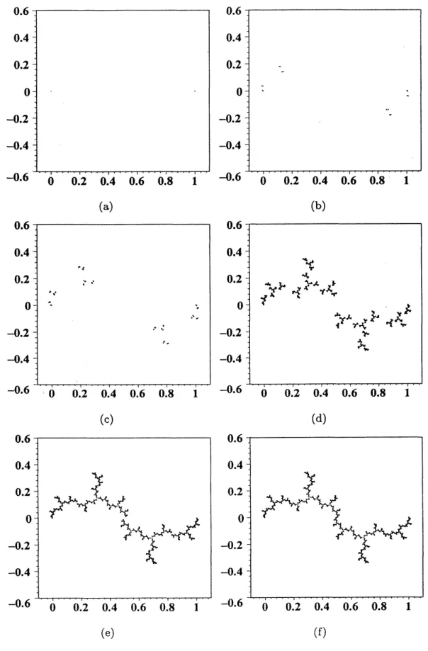
We set $m=12$. Figures 1 $(a)\sim(g)$ show approximations of the Julia set $J(f_{1/\epsilon})$ by

plotting the union of solutions $\bigcup_{n=0}^{15}z_{n}^{*}(\epsilon)$ for six different values of $\epsilon$ integrated along

the ray $\mathcal{R}^{+}(16;M_{\mu}^{-1})$. The six values of $\epsilon$ are (a) $0,$ $(b)0.129889641+0.141065491i,$ $(c)$

$0.233392345+0.176828347i,$ $(d)0.312689831+0.154912018i,$ $(e)0.312597233+0.150118104i$ , (f) $\frac{-i+i\sqrt{1-4i}}{4}$.

4.2

External angle

1/128

Here, we demonstrate how (3) can be employed to obtain periodic orbits for one of the

Misiurewicz points of angle 1/128, $\epsilon\approx 0.567999678+0.348835133i$_. We choose our _initial

condition for (5) to be $\{z_{0}^{*}(0), z_{1}^{*}(0), \ldots, z_{97}^{*}(0)\}=$

{

$0,1,0,0,0,1,1,0,1,1,0,0,0,0,0,1,0,1,0,0,1,1,1,0,0,1,0,1,1,1$

,

$0,1,1,1,0,0,0,0,0,0,0,1,0,0,1,0,0,0,1,1,0,1,0,0,0,1,0,1,0,1$

, 1,

_{$0,0,1,1,1,1,0,0,0,1,0,0,1,1,0,1,0,1,0,1,1,1,1,0,0,1,1,0,1$}

, 1, 1, 1,$0,1,1,1,1\}$,

and perform the numerical integration along the parameter ray $\mathcal{R}^{+}(1\prime 128;M_{\mu}^{-1})$.

Table 1 displays the orbit points together with the numerical

errors

for the obtained

period-98 orbit. It is clear that the errors are within the order of $10^{-5}$.

References

[1] S. AUBRY AND G. ABRAMOVICI, Chaotic trajectories in the standard map: the

concept

_of

anti-integrability, Physica $D,$ $43$ (1990), pp. 199-219.

[2] L.

CARLESON

AND T. W. GAMELIN, Complex Dynamics, Springer-Verlag, New

York, 1993.

[3] Y.-C. CHEN, Bemoulli

_{shift for}

second order

recurrence

relations

near

the

anti-integmble limit, Discrete Contin. Dyn. Syst. $B,$ $5$ (2005), pp.

587-598.

[4] Y.-C. CHEN, Smale horseshoe via the anti-integrability, Chaos Solitons&Fractals,

28, (2006), pp. 377-385.

[5] Y.-C. CHEN, Anti-integmbility

_for

the logistic maps, Chinese Ann. Math. $B,$ $28$

(2007), pp. 219-224.

[6] Y.-C. CHEN, Family

_of

invariant Cantor sets as orbits

_{of differential}

equations, Int.

J. Bifurcat. Chaos,

18

(2008), pp.

1825-1843.

[7] Y.-C. CHEN, T. KAWAHIRA, H.-L. LI, AND J.-M. YUAN, (2009) $2D$ and $3D$

animations available online at http:$//www$.math.sinica.edu.tw$/ycchen/Animations/$.

[8] Y.-C. CHEN, T. KAWAHIRA, H.-L. LI, AND J.-M. YUAN, Family

of

invariant

Cantor sets as orbits

_{of differential}

equaitons. $\Pi$; Julia sets, (2010), Preprint.

[9] A. DOUADY AND J. H. HUBBARD, Iteration des polynomes quadmtiques complexes,

C. R. Acad. Sci. Paris Ser. I Math., 294 (1982), pp. 123-126.

[10] A. DOUADY AND J. H. HUBBARD, Etude dynamique des polynomes complexes.

Partie $I$, Publications Mathematiques d’Orsay, 84-2, 1984.

[11] T. KAWAHIRA, OTIS, (2008), Java applet, available online at

[12] M. LYUBICH, Some typical properties

_of

the dynamics

_of

mtional mappings, Russian

Math. Surveys, 38 (1983), pp. 154-155.

[13] R. S. MACKAY AND J. D. MEISS, Cantori

for

symplectic maps

near

the

anti-integmble limit, Nonlinearity, 5 (1992), pp. 149-160.

[14] R. $MA\tilde{N}E’$, P. SAD, _AND D. SULLIVAN, On the dynamics

of

mtional maps, Ann.

Sci. Ecole Norm. Sup., (4) 16 (1983), pp. 193-217.

[15] J. MILNOR, Dynamics in One Complex Variable, 3rd ed., Annals of Mathematics

Studies, 160, Princeton University Press, Princeton, NJ,

2006.

[16] S. MOROSAWA, Y. NISHIMURA, M. TANIGUCHI AND T. UEDA, Holomorphic

(a) (b)

(c) (d)

(e) (f)

Figure 1: The Julia set $J(f_{1/\epsilon})$ for six different values of $\epsilon$ along $\mathcal{R}^{+}(1/6;M_{\mu}^{-1})$. See also