GRUSIN OPERATOR AND HEAT KERNEL OF NILPOTENT LIE GROUPS(Developments of Cartan Geometry and Related Mathematical Problems)

GRUSIN OPERATOR AND HEAT KERNEL

ON NILPOTENT LIE GROUPS

東京理科大学理工学部古谷賢朗 (KENRO FURUTANI)

DEAPRTMENT OF MATHEMATICS FACULTY OF SCIENCE AND TECHNOLOGY

SCIENCE UNIVERSITY OF TOKYO

兵庫県立大学大学院物質理学研究科岩崎千里 (CHISATO IWASAKI)

DEPARTEMNT OF MATHEMATICS

SCHOOL OF SCIENCE HYOGO UNIVERSITY

ABSTRACT. Thepurposeof this noteis to overviewhowwe canconstructtheheat kernel

for (sub)-Laplacian inariexplicit (integral) form with specialfunctions. Ofcoursesuch

cases will be highlylimited. Nevertheless therewill be lots ofoperators interesting on

nilpotentLie groups. Wewillconcentratefor theoperatorsonnilpotentLie groupsand

their quotient spaces. Here weonly treat with typical low-dimensionalcases. So first

we discussthe heat kernel forGrusin operator in relation with the Mehler formulaand Hamilton-Jacobi thoory and explain a general integral form of heat kernelonnilpotent

Liegroupsfrom this point of view. And thenwestatearelation between the heat kernel

on Heisenberggroupand that forGrusinoperator. Alsoweconstruct anclassical action integral forahigher stepGrusinoperator.

CONTENTS

1. Introduction 1

2. Grusin operator 3

3. Heat kernel

on

nilpotent

groups

5

4. Heisenberg group and Grusinoperator 6

5. Higher step Grusin operator 7

References 11

1. INTRODUCTION

It is known in the statistical mechanics that the heat kernel $K_{t}(x,y)$ is expressed

as

a

path integral

$K(t,$x,$y)= \int_{P_{t}(x,y)}e^{-s_{t(\gamma)}}d\mu(\gamma)$,

2000 Mathematics Subject _{Classification.} 35K05,22E25.

hopefully with a suitable

_ltinfinite

dimensionalmeasure”$d\mu(\gamma)$, where$P_{t}(x, y)$ denote the

path space connecting $x$ to $y$ at a time $t$ and the function $S_{t}(\gamma)$ is called the classical

action and is given by

$S_{t}( \gamma)=1/2\int_{0}^{t}||\dot{\gamma}(s)||^{2}ds$.

By normalizing the time parameter $t=1$, this is also written as

$\frac{1}{t^{N}}\int_{P_{1}(x,y)}e^{-\frac{S(\gamma)}{2t}}d\mu(\gamma),$ $(\gamma_{t}(\sigma)=\gamma(\sigma t))$

and in theLaplacian

case

it has

an

asymptotic expansion

$K(t, x, y) \sim\frac{1}{(2\pi t)^{n/2}}e^{-\mathrm{A}^{x_{\#^{\mathrm{L}^{2}}}}}u_{0}(x, y)(1++O(t))$

.

Here $d(x, y)$ denotesthe Riemanian distance of the point $x$and $y$

.

Forthe sub-Laplacian

cases the small time asymptotic expansion is morecomplicated (cf. [2]). There

are

inter-estingargumentswhich will give

us

areductionof thephysicsformula toamathematically

fixed formula in a certain

case

(cf. [13]). Especially, if the space

we are

working on is

Euclidean, then wehave only

one

segment (geodesics) which connects $x$ and $y$, and the

path integral will reduce tojust a

function

$\frac{1}{(2\pi t)^{n/2}}e^{-\rfloor 1_{A}^{x}\rfloor \mathrm{L}^{2}}\sim$,

the heat kernel of the Laplacian $\Delta=-\frac{1}{2}\sum_{i=1}^{n}\frac{\partial^{2}}{\partial x_{i}^{2}}$

.

It

was

the first in the paper [12] that by a probabilistic argument the heat kernel of

the sub-Laplacian

on

threedimensional Heisenberggroup

was

given inanexplicit integral

formula, and then many papers were published to express the heat kernel for Laplacians

and sub-LaplaciansonnilpotentLiegroups(see [1], [2], [3], [15] and also recent papers [13],

[5]

or

[6] for dealing with similar subject and calculations). In

case

of the sub-Laplacian

we

will necessarily have

an

integral expression for the heat kernel,

even

if it reduces to

a

fixed finitedimensional integral expressionsince there

are many

geodesics connecting two

points even locally. The first step ofthis is how

we can

suppose that the formula looks like?

So in

\S 2

we explain the case of Grusin operator $\mathcal{G}=-\frac{1}{2}(\frac{\partial^{2}}{\partial x^{2}}+x^{2}\frac{\partial^{2}}{\partial y^{2}})$ following a

standard way ofthespectral decomposition ofselfadjoint operators and arrive at a form

as a

natural conclusion. Then we discuss the functions in the formula from

Hamilton-Jacobi theory. In

\S 3

we state apossible formula for the heat kernel on general nilpotent

Lie groups and explain an action integral and transport equation which will be satisfied

by the functions appearing inthe formula. In

\S 4 we

give

a

relation between heat kernels

on

Heisenberg group and Grusin operator in terms of fiber integration. Finally in

\S 5

we

solve

a

Hamilton system for

a

higher step Grusin operator and construct

an

action

2. GRUSIN OPERATOR

Let $\mathcal{G}=-\frac{1}{2}(\frac{\partial^{2}}{\partial x^{2}}+x^{2}\frac{\partial^{2}}{\partial y^{2}})$ be Grusin operator and denote by $F:L_{2}(\mathbb{R}^{2}, dxdy)arrow L_{2}(\mathbb{R}^{2}, dxd\eta)$

$\mathcal{F}(\varphi)(x, \eta)=\int_{\mathrm{R}^{2}}e^{-\sqrt{-1}y\eta}\varphi(x,y)dy$

apartial Fouriertransformation.

Through thispartial Fourier transformation, Grusin operator $\mathcal{G}$ is

seen as

$\mathcal{L}=-\frac{1}{2}(\frac{\partial^{2}}{\partial x^{2}}-x^{2}\eta^{2})$ ,

acting

on

$L_{2}(\mathbb{R}^{2}, dxd\eta)$. When

we

regard the variable

$\eta$

as

a constant, the heat kernel $\mathcal{L}_{\eta}(t, x,x)\wedge$ of the operator

$L_{\eta}=- \frac{1}{2}(\frac{\partial^{2}}{\partial x^{2}}-x^{2}\eta^{2})$

for $\eta\neq 0$is expressed asthe

sum

of eigenfunctions $V_{n}(x)$ $(L_{\eta}V_{n})(x)= \frac{(2n+1)|\eta|}{2}V_{n}(x)$,

where

$V_{n}(x)=e^{-1/2|\eta|x^{2}}H_{n}(\sqrt{|\eta|}x)$

and

$H_{n}(x)=(-1)^{n}e^{x^{2}} \frac{d^{n}e^{-x^{2}}}{dx^{n}}$

isthe n-th Hermite polynomial:

$\mathcal{K}_{\eta}(t, x, x)\wedge=\sum_{n=1}^{\infty}e^{-\frac{2n\neq 1}{2}|\eta|t_{\frac{\sqrt{|\eta|}V_{n}(x)V_{n}(_{X}^{\wedge})}{\sqrt{\pi}2^{n}n!}}}$

(2.1) $= \sqrt{|\eta|}^{-\frac{1}{2}|\eta|\ell(x^{2}+x^{2})}ee^{-\mathrm{M}_{2}\wedge}\sum\frac{H_{n}(\sqrt{|\eta|}x)H_{n}(\sqrt{|\eta|}x)\wedge}{\sqrt{\pi}2^{n}n!}e^{-nt|\eta|}$

.

Then by the Mehler formula (cf. [17])

we

know that (2.1) equals to

(2.2) $\frac{1}{\sqrt{\pi}}\sqrt{\frac{\eta}{e^{t\eta}-e^{-t\eta}}}e^{-_{4}}\mathrm{n}\{(x+x)^{2}\wedge\tanh_{2}^{x^{t}-}+(x-x)^{2}\coth_{2}^{1^{t}}\cdot\}$

.

Note that $|\eta|\tanh|\eta|=\eta\tanh\eta$ (and so on).

Also we have

$\lim_{\etaarrow 0}\mathcal{K}_{\eta}(t, x, x)\wedge$

$= \lim_{\etaarrow 0}\frac{1}{\sqrt{2\pi}}\sqrt{\frac{\eta}{\sinh t\eta}}e^{-f}4\{(x+x)^{2}\wedge\tanh\doteqdot t+(x-x)^{2}\wedge\coth_{2}^{\mathrm{L}^{\ell}\}_{=\frac{1}{\sqrt{2\pi t}}e^{-\frac{|*-\epsilon_{\mathrm{I}^{2}}}{2t}}}}$

is theheat kernel for the $\mathrm{o}\mathrm{p}\mathrm{e}\mathrm{r}\mathrm{a}\mathrm{t}\mathrm{o}\mathrm{r}-\frac{1}{2}\frac{d^{2}}{dx^{2}}$

.

Now we have the heat kernel $K^{Q}=K\sigma(t, x, y,x, y)\wedge\wedge$ ofthe Grusin operator $\mathcal{G}=F^{-1}\circ$

$\mathcal{L}\circ F$;

$(e^{-t\mathcal{G}}f)(x, y)= \int K^{g}(t, x, y,xy)\wedge,$$\wedge f(xy)\wedge,$$\wedge d_{X}^{\wedge}dy;\wedge$

$K\sigma(t, x, y,xy)\wedge,\wedge$

(2.3) $= \frac{1}{(2\pi)^{3/2}}I^{e^{\sqrt{-1}\eta}e^{-f}}(v-y)\wedge\{4(x+^{\wedge}x)^{2}\tanh_{2}^{\Delta}t+(x-x)^{2}\wedge\coth_{2}^{\Delta}\}t\sqrt{\frac{\eta}{\sinh t\eta}}d\eta$

.

In the above expression, ifwe still change the variable $t\eta$to $\eta$ (

$=\mathrm{t}\mathrm{i}\mathrm{m}\mathrm{e}$ rescaling), then

it becomes the following form:

$K(t, x,y,xy)\wedge,\wedge$

(2.4) $= \frac{1}{(2\pi t)^{3/2}}\int e^{\frac{\sqrt{-1}(y-y)\wedge\eta}{t}}e^{-L\{(x)^{2}\tanh_{2}^{f}+(x-x\rangle^{2}\coth_{2}^{f}\}}4tx+^{\wedge}\wedge\sqrt{\frac{\eta}{\sinh\eta}}d\eta$.

Put

$S(x, x, \eta)\wedge=\frac{\eta}{4}\{(x+x)^{2}\wedge\tanh\frac{\eta}{2}+(x-x)^{2}\wedge\coth\frac{\eta}{2}\}$

and $V(\eta)=\sqrt{\frac{\eta}{\sinh\eta}}$, and then

we

write this integral form (2.4)

as

(2.5) $\frac{1}{(2\pi t)^{3/2}}\int e\iota\sqrt{-1}^{1L^{-}\text{\^{u}}\ln}e^{-\frac{s(x,x_{j}\eta)\wedge}{t}}V(\eta)d\eta$

.

Now

we

construct the function $S=S(x,x;\eta)\wedge$ by solving aHamilton system with the

Hamiltonian $2H^{\eta}=2H^{\eta}(x, \xi)=\xi^{2}-x^{2}\eta^{2}$:

(2.6) $\{$

$\xi(s)=\frac{\frac{\partial}{-}\partial H^{\eta}j_{H^{\eta}}}{\partial x}=x\eta^{2}x:(s)==\xi,$

,

boundary condition:$x(\mathrm{O})=x,$ $x(t)=x\wedge$.

In fact this system is solved explicitly with the solutionthat

$x(s)=x(s;t, x, x, \eta)\wedge=\frac{\wedge x\sinh s\eta+x\sinh\eta(t-s)}{\sinh t\eta}$

$\xi(s)=\xi(s;t, x,x\eta)\wedge,=\dot{x}(s)=\eta\frac{x\cosh\wedge s\eta-x\cosh(t-s)\eta}{\sinh t\eta}$,

for any $t,$$x,$$x\wedge\in \mathbb{R}$

.

With this solution, let _{$\varphi=\varphi(x,x,t;\eta)\wedge$} be the integral (2.7) $\varphi(x,xt;\eta)\wedge,=\int_{0}^{t}\dot{x}(s)\xi(s)-H^{\eta}(x(s),\xi(s))ds$.

Thisintegral is called

a

classical action and is equal to

$\varphi(x,xt;\eta)\wedge,=\eta^{2}\int_{0}^{\ell}x^{2}(s)ds+\frac{t}{2}E$

where the constant

$E\equiv\xi^{2}(s)-x^{2}(s)\eta^{2}=\xi^{2}(0)-x^{2}\eta^{2}$

$= \frac{\eta^{2}\{4(x^{2}+x^{2})\wedge 4xx(\wedge e^{t\eta}+e^{-t\eta})\}}{(e^{t\eta}e^{-t\eta})^{2}}=$

is an invariant of the Hamilton system (2.6).

Here

we

know that the function $\varphi(x, x, 1\wedge;\eta)$ coincides with the function $S$ and it is

a

solution of the Hamilton-Jacobiequation:

(2.9) $\frac{\partial}{\partial t}\varphi(x, x, t;\eta)\wedge+H^{\eta}(x\frac{\partial}{\partial_{X}^{\wedge}}\wedge,\varphi(x, x, t;\eta)\wedge)=0$

.

The function $\varphi$ has aproperty that $\varphi(x,x, 1\wedge;t\eta)=t\varphi(x,xt;\eta)\wedge,$, and this implies that

thefunction $S$satisfies the equation, called generalized Hamilton-Jacobi equation:

(2.10) $H^{\eta}(x, \frac{\partial}{\partial_{X}^{\wedge}}\wedge S(x,x\eta)\wedge,)+\eta\frac{\partial}{\partial\eta}S(x, x, \eta)\wedge=S(x,x, \eta)\wedge$

.

For each fixed $t,$ $x$ and $\eta$ let

$\mathcal{V}$ _{$:\wedge x->\xi(0;t, x, x, \eta)\wedge$}, then by the explicit expression of

thesolution of the Hamilton system

we

have

(2.11) $\mathcal{V}(x)\wedge=\frac{\eta}{\sinh t\eta}(x-\wedge x\cosh t\eta)$,

and

(2.12) $\sqrt{\frac{\partial \mathcal{V}}{\partial_{X}^{\wedge}}(x)\wedge}=\sqrt{\frac{\eta}{\sinh t\eta}}$

.

This function $\sqrt{\frac{\partial \mathcal{V}}{\partial_{X}^{\wedge}}}$

, as a function of the parameter $\eta$ (with $t=1$), is a solution of the

transport equation (3.6)(see

_{\S 3).}

Summing up,

we

know that the functions in the integral form (2.3) coincide with the

functions (2.8) and (2.12)

we

constructed by solving the Hamilton system (2.6). In fact

by putting $t=1$ (time rescaling) wehave the functions$S=S(x,x, \eta)\wedge=\varphi(x_{0}, x, 1;\eta)$and

$\sqrt{\frac{\partial \mathcal{V}}{\partial_{X}^{\wedge}}(x)\wedge}=V(\eta)(\mathrm{c}\mathrm{f}. [18], [10])$

.

3. HBAT KERNEL ON NILPOTENT GROUPS

Onthe Liegroup$G$theheat kernelfor the(left)invariant (sub)-Laplacian$\Delta=-\frac{1}{2}\sum\tilde{X}_{i}^{2}$

takes theform $k(t, g^{-1}\cdot h)$ with

a

smoothfunction $k(t, g)\in C^{\infty}(\mathbb{R}_{+}\cross G)$satisfying

(3.1) $( \frac{\partial}{\partial t}+\Delta)k(t,g)=0$

(3.2) $\lim_{t\downarrow 0}k(t, g)=\delta_{\mathrm{e}},$

$\delta_{e}$ isthe

6

function at the identity element $e\in G$

.

So, ifthe heat kernelwould be given by a function$k(t,g)$ ofan integral form

(3.3) $\frac{1}{t^{N}}\int e^{-\underline{X}\mathrm{t}1}V(g, \eta)\mathit{4}_{\ell}\Delta d\eta$

witha function$f=f(g, \eta)\in C^{\infty}(G\mathrm{x}\mathbb{R}^{t})$ which wetake

a

functiondefinedbythe integral

similar to (2.7) with

a

modification of the term $\sqrt{-1}(y-y)\wedge\eta$ (we call $f$

a

complex action

function), then the function $V=V(g,\eta)$ (we call it a volume element) will satisfy

an

equation (called transport equation).

Now

we

shall statetheseequations. Let $H$be theHamiltonianof the (sub)-Laplacian$\Delta$

and the function $f$ satisfies the equation, called generalized Hamilton-Jacobi

equa-tion:

(3.4) $H(x, \nabla f)+\sum\eta_{i}\frac{\partial}{\partial\eta_{i}}f(x, \eta)=f(x, \eta)$

.

And then with one solution of this equation

we assume

that the function $V$ satisfy the

equation, called transport equation:

(3.5) $\sum\eta_{i^{\frac{\partial V}{\partial\eta_{i}}+}}(\sum_{i}\tilde{X}_{i}(f)\tilde{X}_{\dot{*}}(V)-(\Delta(f)+N-\ell)\cdot V)=0$

.

Especially, if the function $V$ does not depend

on

the space variables then, this equation

reduces to

(3.6) $\sum\eta_{i^{\frac{\partial V}{\partial\eta_{1}}-}}(\Delta(f)+N-\ell)V=0$.

The function (2.12) is a solutionofthisequation.

If

we

have these two functions $f$ and $V$ satisfying the generalized Hamilton-Jacobi

equation and transport equation then these will give the heat kernel. In the paper[1] it

wasprovedthatfor thesub-Laplacian

on

anytwo step nilpotent Lie groupthe heat kernel is given by the integral (3.3) with acomplex action $f$ and aavolume element $V$

.

In fact

both of them are explicitly given in _{terms of hyperbolic functions. The complex action}

functionisconstructedbysolving

a

Hamilton system ($\sim \mathrm{b}i$-characteristicequation) under

initial-boundaryconditions and the volume element is constructed from the Jacobian of

the correspondence similar to the map (2.11) _{between boundary condition and initial}

condition ofthe Hamilton system (see [8] for

an

aspect offunctional calculus).

4. HEISENBERG GROUP AND GRUSIN OPERATOR

Inthe this section wejust describe the heat kernel of the three dimensional Heisenberg

group and discuss

a

relation with that for Grusin operator. Let$\mathrm{H}$be the three dimensional Heisenberggroupanddenote

its Lie algebra by$\mathfrak{h}$whose

basis wedenote by

{X,

$\mathrm{Y},$ $Z$

}

with the bracket relation

$[x_{-},\mathrm{Y}]_{-}=Z$

.

We identify $\mathrm{H}$ and

$\mathfrak{h}$ throughthe exponentialmap$\mathrm{e}\mathrm{x}\mathrm{p}:\mathfrak{h}arrow \mathrm{H}$ anddenote by $X,$ $\mathrm{Y}$and $\overline{Z}$

theleft invariant

vector fields corresponding to $X,$ $\mathrm{Y}$ and _$Z$ respectively. Then

$\Delta_{sub}=-\frac{1}{2}(\tilde{X}^{2}+\tilde{Y}^{2})$ is

a

sub-Laplacian

on

H. Let $\mathrm{N}_{Y}=[\{t\mathrm{Y}\}_{t\in \mathrm{R}}]$ be

a

subgroup generated by the element Y.

The map$\rho:\mathrm{H}arrow \mathbb{R}^{2}$defined by

$\rho:\mathrm{H}\cong \mathfrak{y}\ni g=xX+y\mathrm{Y}+zZ=(x, y, z)\mapsto(u,v)\in \mathbb{R}^{2}$

$u=x,$ $v=z+ \frac{1}{2}xy$

realizesthe projection map

$\mathrm{H}\cong \mathbb{R}^{3}arrow \mathrm{N}_{Y}\backslash \mathrm{H}\cong \mathbb{R}^{2}$.

In fact, this is a principal bundle and the trivialization is given by the map

$\mathrm{N}_{Y}\cross(\mathrm{N}_{Y}\backslash \mathrm{H})\cong \mathbb{R}\cross \mathbb{R}^{2}\ni(a,\cdot u, v)\mapsto(x, y, z)\in \mathbb{R}^{3}\cong \mathrm{H}$

(4.1) $(a;u, v)->(u, a, v- \frac{1}{2}au)$_.

Then the left invariant vector field$\tilde{X}=\frac{\partial}{\partial x}-\frac{y}{2}\frac{\partial}{\partial z}$descends to thevectorfield

$\frac{\partial}{\partial u}$ and

$\overline{Y}=\frac{\partial}{\partial y}+\frac{x}{2}\frac{\partial}{\partial z}$descends to

$u \frac{\partial}{\partial v}$. So the sub-Laplacian $\Delta_{\epsilon ub}$ on$\mathrm{H}$ and

Grusin

operator

commutes eachother through the map $\rho$:

(4.2) $\Delta_{\epsilon ub}\circ\rho^{*}=\rho^{*}\circ \mathcal{G}$

.

By the left invariance of$\Delta_{sub}$, the heat kernel $K^{\mathrm{H}}(t;g, h)\in C^{\infty}(\mathbb{R}+\mathrm{x}\mathrm{H}\mathrm{x}\mathrm{H})$ of $\Delta_{sub}$

takestheform$K^{\mathrm{H}}(t;g, h)=k^{\mathrm{H}}(t;g^{-1}\cdot h)$with

a

smooth function$k^{\mathrm{H}}(t, g)\in C^{\infty}(\mathrm{R}_{+}\cross \mathrm{H})$

.

This function is given

as

(cf. [1]):

(4.3) $k^{1\mathrm{I}}(t,g)=k^{\mathrm{H}}(t, x,y, z)= \frac{1}{(2\pi t)^{2}}\int e^{-\frac{\sqrt{-1}\eta*\S rn\mathrm{t}\mathrm{h}\mathrm{g}.(ae^{2}+y^{2})}{\mathrm{t}}}\frac{\eta}{2\sinh_{2}^{f}}d\eta$

Now by (4.1) and (4.2)

we

have

$\int_{-\infty}^{+\infty}K^{\mathrm{H}}(t, (x, y, z), (u, a, v-1/2ua))da$

$=K^{\mathcal{G}}(t, (x, z+1/2xy), (u, v))$

that is, thefiber integration of the function$K^{\mathrm{H}}(t;g, h)$ alongthe fiber of the map $\rho$gives

theheat kernel oftheGrusin operator.

5. HIGHER STEP GRUSIN OPERATOR

Higher step Grusin operator is defined

as

(5.1) $\mathcal{G}^{(k)}=-\frac{1}{2}(\frac{\partial^{2}}{\partial x^{2}}+x^{2k}\frac{\partial^{2}}{\partial y^{2}})$

.

All these

comes

fromasub-Laplacianon asuitable nilpotent Lie group$\mathrm{G}_{k+1}$, i.e.,let$\mathfrak{g}_{k+1}$

be

a

Lie algebra with the basis $\{X_{0}, \cdots , X_{k}\}$ such that bracket relations are defined by

$[X_{0},X_{1}]=X_{2},$ $[X_{0}, X_{2}]=X_{3},$$\cdots,$$[X_{0}, X_{k-1}]=X_{k},$ $[X_{0},$$X_{k}|=0$,

andall other

are

zero.

$\mathrm{G}_{k+1}$ is the corresponding simplyconnected group and

we

identify

it with $\mathrm{g}_{k+1}$ through the exponential map.

Let$N$be

a

subgroupof$\mathrm{G}_{k+1}$ generatedby$\{X_{1}, \cdots,X_{k-1}\}$, then$N\backslash \mathrm{G}_{k+1}$is isomorphic

to$\mathbb{R}^{2}$ and the sub-Laplacian

on

$\mathrm{G}_{k+1}$

$- \frac{1}{2}(\tilde{X}_{0}^{2}+\overline{X}_{1}^{2})$

descends to

$- \frac{1}{2}(\frac{\partial^{2}}{\partial x^{2}}+x^{2k}\frac{\partial^{2}}{\partial y^{2}})$

.

This group is aspecial class of

Carnot

group (cf. [5]), and Engelgroup is such an

one

of

dimension 4 (we ignore

a

constant infront of$x^{2k}$).

Until

now

we have no explicit expression for the heat kernel

on

nilpotent Lie group of

step greater than 3. In this final section we construct the classical action integral of a

higher step Grusin operator

$\mathcal{G}^{(2)}=-\frac{1}{2}(\frac{\partial^{2}}{\partial x^{2}}+x^{4}\frac{\partial^{2}}{\partial y^{2}})$.

Through the partial Fourier transformation,1‘

we

_{consider theoperator (cf. [19], [20])}

$L_{\eta}^{(2)}=- \frac{1}{2}(\frac{\partial^{2}}{\partial x^{2}}-x^{4}\eta^{2})$

.

As in

\S 1,

for each fixed $\eta\neq 0$the heat kernel$\mathcal{K}^{L_{\eta}^{(2)}}(t, x,x)\wedge$ of the

operator $L_{\eta}^{(2)}$ has a form $\mathcal{K}\iota_{\eta}^{(2)}(t,x,x)\wedge=\sqrt{|\eta|}\cdot\Sigma e^{-t(\nu\overline{|\eta|})^{\mathrm{z}_{\lambda_{k}}}}\varphi_{k}(\sqrt{|7||}x)\varphi_{k}(\sqrt{|\eta|}\overline{x})$

with the normalized eigenfunctions of$L_{1}^{(2)}$:

$(L_{1}^{(2)}\varphi_{k})(x)=\lambda_{k}\varphi_{k}(x),$ $0\leq\lambda_{1}\leq\lambda_{2},$ $\cdots$ , $\int|\varphi(x)|^{2}dx=1$

.

The heat kernel of

a

higher step Grusin operator

.

$\mathrm{r}-1_{\circ \mathcal{G}_{2}\mathrm{o}F}=-\frac{1}{2}(\frac{\partial^{2}}{\partial x^{2}}+x^{4}\frac{\partial^{2}}{\partial y^{2}})$ will

be

$\frac{1}{2\pi}\int e^{\sqrt{-1}(y-y)\eta}\mathcal{K}^{L_{\eta}^{(2)}}(t, x, x)\wedge d\eta\wedge$.

It is not clear that this has

a

similar

_form

with (2.3)

or

(2.4). We construct here an

action integral by solving

a

Hamilton system similar to (2.6), which solution is given in

terms

_of

elliptic

_functions

and

we

will know that the action integral

_satisfies

Hamilton-Jacobi equation.

Let $H^{\eta}=H^{\eta}(x, \xi)=\frac{1}{2}(\xi^{2}-x^{4}\eta^{2})$ be the Hamiltonian of the operator $L_{\eta}^{(2)}$, and $\mathrm{c}o$nsider the Hamilton system:

$\dot{x}(s)=\xi,\dot{\xi}(s)=-H_{x}^{\eta}(x, \xi)=2x^{3}\eta^{2}$

with the boundary condition

$x(\mathrm{O})=x_{0},$ $x(t)=x,$ ( $x_{0},$ $x$ and $t\neq 0$ should be taken arbitrary).

The system reduces to

a

single non-linear equation:

(5.2) $\ddot{x}=2x^{3}\eta^{2}$, with the boundarycondition _{$x(\mathrm{O})=x_{0},$ $x(t)=x$}

.

It is enough to consider the

cases

except $x_{0}=0=x$, for which

we

have the trivial

solution $x(s)\equiv 0$

.

Then, by the transformations $srightarrow t-s$ and $x(s)rightarrow-x(s)$, it is

enough to consider the two

cases

of the boundary data with $t>0$:

(I) $x_{0}\leq 0<x$,

(II) $0<x_{0}\leq x$

.

We describe the solution:

Case I. Let $x_{0}\leq 0<x$

.

Let $F_{\lrcorner}>0$ and the function $h(y, E)$ be

$h(y, E)= \int_{x_{0}}^{y}\frac{du}{\sqrt{u^{4}\eta^{2}+E}}$ ,

then for each fixed $y$ the function $h(y, E)$ is monotone as a function of $E>0$, and for

each fixed $x>0\geq x_{0}$ it takes values from $0$ to

oo

when $E$

moves

from oo to $0$

.

So put

$E=E(x_{0}, x, t;\eta)$ be the unique constant such that

$\int_{x_{0}}^{x}\frac{du}{\sqrt{u^{4}\eta^{2}+E}}=t>0$

.

Nowsincethefunction$h(y, E(x_{0}, x,t;\eta))(-\infty<y<+\infty)$ismonotone,let$x(s;E(x_{0},x,t;\eta))$

be its inverse function, i.e.,

$\int_{x\mathrm{o}}^{x(\epsilon;E(x\mathrm{o},x,t_{j}\eta))}u^{4}\eta^{2}+E=(x_{0}, x, t;\eta)du=s$,

then $x(s:E(\prime x_{0}, x, t;\eta))$ is the unique solution of the equation (5.2).

Case II. Let $0<x_{0}\leq x$

.

Then we need to divide into three

cases.

II-1. Let $0<t \leq\frac{x_{0}^{-1}-x^{-1}}{|\eta|}=\int_{x_{0}}^{x}\frac{du}{\sqrt{u^{4}\eta^{2}}}$.

Then for such $t$ and _{$x>x_{0}$}

we

have

a

unique value$E=E(x_{0}, x, t;\eta)\geq 0$ such that

$\int_{x_{0}}^{x}\frac{du}{\sqrt{u^{4}\eta^{2}+E}}=t$

.

The solution$x(s;E(x_{0}, x,t;\eta))$ of (5.2) is then given by the integral

$\int_{x_{0}}^{x(s,E(x_{0},x,\ell;\eta))}u^{4}\eta^{2}+E=(x_{0}, x,t;\eta)du=sdu$.

II-2.

We

aesume

$\frac{x_{0}^{-1}-x^{-1}}{|\eta|}<t\leq\int_{x_{0}}^{x}u^{4}\eta^{2}=^{du}-x_{0}^{4}\eta^{2}$ andfix theuniquevalue$E=E(x_{0}, x,t;\eta)$

$(0>E\geq-x_{0}^{4}\eta^{2})$ such that $\int_{x0}^{x}u^{4}\eta^{2}+E=(x_{0}, x,t;\eta)du=t$, then the solution of (5.2) is

given by

$\int_{x\mathrm{o}}^{x(s;E(x0,x,t;\eta))}u^{4}\eta^{2}+E=(x_{0}, x,t;\eta)du=s$

.

II-3.

Then

we

take the unique value $a=a(x_{0}, x, t;\eta)(a(x_{0}, x, t;\eta)$

can

be chosen uniquely

in $0<a(x_{0}, x, t;\eta)<x_{0})$ such that

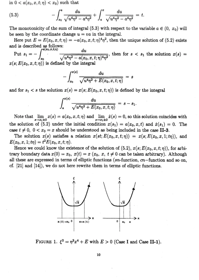
(5.3) $- \int_{x_{0}}^{a}u^{4}\eta^{2}=^{du}-a^{4}\eta^{2^{+}}\int_{a}^{x}u^{4}\eta^{2}=^{du}-a^{4}\eta^{2}=t$.

The monotonicity of the

sum

of integral (5.3) with respect to the variable$a\in(\mathrm{O}, x_{0})$will

be

seen

by the coordinate change$u=va$ in the integral.

Here put $E=E(x_{0}, x, t;\eta)=-a(x_{0}, x, t;\eta)^{4}\eta^{2}$, thenthe unique solution of(5.2) exists

and is described as follows:

Put $s_{1}=- \int_{x0}^{a(x\mathrm{o},x,t;\eta)}u^{4}\eta^{2}-a(=x_{0}, x, t;\eta)^{4}\eta^{2}du$, then for _{$s<s_{1}$} the solution $x(s)=$

$x(s;E(x_{0}, x,t;\eta))$is defined by the integral

$- \int_{x0}^{x(s)}u^{4}\eta^{2}+E=(x_{0}, x, t;\eta)du=s$

and for $s_{1}<s$the solution $x(s)=x(s;E(x_{0}, x,t;\eta))$ is defined by the integral

$\int_{a}^{x(s)}u^{4}\eta^{2}+E=(x_{0}, x, t;\eta)d\mathrm{u}=s-s_{1}$

.

Note that$\lim_{\epsilonarrow s_{1}\pm 0}x(s)=a(x_{0}, x, t;\eta)$ and$\lim_{\epsilonarrow s_{1}\pm 0}\dot{x}(s)=0$,

so

thissolutioncoincideswith

the solution of (5.2) under the initial condition $x(s_{1})=a(x_{0}, x,t)$ and $\dot{x}(s_{1})=0$

.

The

case

$t\neq 0,0<x_{0}=x$should be understood

as

being included in the

case

II-3.

The solution $x(s)$ satisfies

a

relation $x(st;E(x_{0}, x, t;\eta))=x(s;E(x_{0}, x, 1;t\eta))$, and

$E(x_{0}, x, 1;t\eta)=t^{2}E(x_{0}, x, t;\eta)$

.

Hence we couldknow the existence ofthe solution of (5.2), $x(s;E(x_{0}, x, t;\eta))$, for

arbi-trary boundary data$x(\mathrm{O})=x_{0},$ $x(t)=x$ ($x_{0},$ $x,$ $t\neq 0$

can

be takenarbitrary). Although

all these

are

expressed in terms of ellipticfunctions ($sn$-function, $\sigma n$-function and

so

on,

cf. [21] and [14]$)$, we do not hererewrite them in terms of elliptic functions.

FIGURE 1. $\xi^{2}=\eta^{2}x^{4}+E$ with $E>0$ (Case I and Case II-1).

FIGURE 2. $\xi^{2}=\eta^{2}x^{4}+E$ with$E<0$ (Case II-2 and Case II-3).

Now based

on

the existence ofthe solutionof(5.2) we

can

define the (classical) action

integral $f$:

(5.4) $f(x_{0},x,t; \eta)=\int_{0}^{t}\dot{x}(s)\xi(s)-H^{\eta}(x(s),\xi(s))ds$

.

By the relation$\dot{x}(s)^{2}=\eta^{2}x(s)^{4}+E(x_{0}, x, t;\eta)$, this integral equals to

$f(x_{0}, x, t; \eta)=\eta^{2}\int_{0}^{t}x(s)^{4}ds+\frac{t}{2}E(x_{0}, x,t;\eta)$

$= \eta^{2}\int_{x_{0}}^{x}y^{4}\eta^{2}+E=(x_{0}, x,t;\eta)dyy^{4}+\frac{t}{2}E(x_{0}, x, t;\eta)$

(5.5) $= \pm\frac{1}{3}\{x\sqrt{x^{4}\eta^{2}+E(x_{0},x,t;\eta)}-x_{0}\sqrt{x_{0^{4}}\eta^{2}+E(x_{0},x,t;\eta)}\}+\frac{t}{6}E(x_{0},x, t;\eta)$

$(\xi(s)=\dot{x}(s)=\pm\sqrt{x^{4}(s)r_{l^{2}}+E(x_{0},x,t;\eta)})$.

$f$ is

a

solution of Hamilton-Jacobi equation $\frac{\partial}{\alpha}f+H(x, \nabla f)=0$ and also satisfies the

generalized Hamilton-Jacobi equation

$H(x, \nabla f)+\eta\frac{\partial}{\partial\eta}f(x_{0}, x, 1;\eta)=f(x_{0}, x, 1;\eta)$,

which is proved by making use of the relation: $tf(x_{0}, x, t;\eta)=f(x_{0}, x, 1;t7|)$

.

Finally

we

note that our arguments above

are

also valid to show the existence of the

solution for the Hamilton system (5.2) of general higher step Grusin operator and so

we

have

an

action integral similar to (5.5).

REFERENCES

[1] R. Beals, B. Gaveau and P. Grciner : The Green Ihnction _ofModel Step two HwoelliPtic

Oper-ators and the Analysis ofCertain Tangential Cauchy Riemannian Complexes, Advances in Math.

121(1996).

[2] –, –, –: Hamilton-Jacobi Theory and the Heat Kemel on Heisenberg groups, J.

Math. PuresApPl. 79(2000).

[3] –, –, –: Complex Hamiltonian mechanics and parnmetrisesfor subelliptic

[4] –, –,–: On a geometnc

formula

for

thefundamentalsolution ofsubelliptic

Lapla-cians,Math. Nachr. 181 (1996), 81-163.

[5] D. C.uChang and I. Markina : Geometric analysis and Green_function on anisotropic quatemion

Carnot groups, toappcar in AdvancesinAppliedMath.

[6] 0. Calin, D. C. Chang andJ. Tie: Fundamentalsolutions_forHermite andsubelliptic operators to

appear in J. d’Analyse Math.

[7] K.Furutani: The heat kemel and the spectrum

_of

aclass ofntlmanifolds,Comm. Partial Differential

Equations, 21,No. 3&4 (1996),423-438.

[8] –: Heat Kemels _ofthe sub-Laplacian and the Laplacian on Nilpotent Lie Groups, to appear

in Analysis, Geometry and Topology of Elliptic Operators, Papers in honour of KrzysztofP.

Woj-ciechowski,pp. 185-226,WorldScientific,London-Singapore(2006).

[9] B. Gaveau : Principe de moindre action,propagation de la chdeur et estimees sous-elliptiques sur

certainsgroupes nilpotents,ActaMath. 139 (1977),95-153

[10] M. de Gosson : The Principles

_of

Newtonian and Quantum Mechanics, Imperial College Press,

London, 2001.

[11] P.Greiner: On the heatkefnel volume element, 2000 (unpublished manuscript).

[12] A. Hulanicki: The distfibution

_of

enem

intheBrownian motion in the Gaussian_fieldand

andytic-hypoellipticity_ofcertain subelliptic opemtors onthe Heisenberggroup, Studia Math. 56 (1976),

165-173.

[13] A. Klinger : New derivation

_of

the Heisenberg kemel, Comm. Partial Differential Equations 22

(1997), 2051-2060.

[14] D. F. Lawdcn : Elliptic R4nction and Applications, Applied MathematicalSciences 80,

Springer-Verlag (1989).

[15] L.P.Rothshild and E.M. Stein: Hypoelliptic_DifferentialOperators and Nilpotent Lie Groups,Acta

Math. 137, No.3/4 (1976), 247-320.

[16] R. S. Strichartz : Sub-Riemannian Geometry,J. Differential Geom., 24, No 2 (1986),221-263.

[17] S. Thangavelu : Lectures on Hermite and Laguerre $Ex\mu nsions$, Mathematical Notes 42 (1993),

Princcton Universitypress

[18] J. H.vanVleck: The$\omega f+esponden$ceprinciPle inthe statistical interpretationofquantum mechanics,

Proc. Natl.Acad. Sci. U.S.A. 14, No. 176 (1928), 178-188.

[19] A. Voros : Zeta

_functions

_ofquartic (and homogeneous $anharmon\dot{l}C$) oscillators, LectureNotes in

Math.,925,Springer (1982), 184-208.

[20] –: Theretum_ofthe quartic oscillator. The complex WKBmethodAnn.Inst. HenriPoincar6

39,No. 3 (1983), 211-338.

[21] E. T. Whittaker and G. N. Watson : A Course _ofModem Analysis, Cambridge University Press