Detection of 3D points on moving objects from point cloud data for 3D modeling of outdoor environments

全文

(1)DETECTION OF 3D POINTS ON MOVING OBJECTS FROM POINT CLOUD DATA FOR 3D MODELING OF OUTDOOR ENVIRONMENTS Tsunetake Kanatani†,‡, Hideyuki Kume‡, Takafumi Taketomi‡, Tomokazu Sato‡ and Naokazu Yokoya‡ †Hyogo Prefectural Institute of Technology 3-1-12 Yukihira, Suma, Kobe, Japan ‡Nara Institute of Science and Technology 8916-5 Takayama, Ikoma, Nara, Japan ABSTRACT A 3D modeling technique for an urban environment can be applied to several applications such as landscape simulations, navigational systems, and mixed reality systems. In this field, the target environment is first measured using several types of sensors (laser rangefinders, cameras, GPS sensors, and gyroscopes). A 3D model of the environment is then constructed based on the results of the 3D measurements. In this 3D modeling process, 3D points that exist on moving objects become obstacles or outliers to enable the construction of an accurate 3D model. To solve this problem, we propose a method for detecting 3D points on moving objects from 3D point cloud data based on photometric consistency and knowledge of the road environment. In our method, 3D points on moving objects are detected based on luminance variations obtained by projecting 3D points onto omnidirectional images. After detecting 3D the points based on evaluation value, the points are detected using prior information of the road environment. Index Terms— Outdoor Environment, 3D Modeling, 3D Point Cloud Data, Moving Objects, HSV Model 1. INTRODUCTION 3D models reconstructed based on measurements of the real world are used for various applications such as landscape simulations, navigational systems, and mixed reality systems. One way to create a 3D model is through a manual reconstruction using 3D modeling software. However, for urban 3D modeling, manual reconstruction involves a considerable amount of work and time. To reduce the effort required for 3D modeling, several automatic reconstruction techniques have been proposed. 3D reconstruction using an image sequence is one automatic reconstruction method utilized [1][2][3]. Such methods can automatically create a large-scale 3D model of a real environment. However, a lot of images are required to construct a high-quality 3D model. On the other hand, 3D modeling methods based on measurements from several different sensors have also been developed [4][5][6][7][8]. One of the advantages of such. Range data Moving object. Unmeasured area. B Moving object. Unmeasured area. A. Fig. 1. Example of data measured using a mobile mapping system sensor-based methods is the accuracy of the measurement. A sensor-based method can obtain the precise shape of a real environment using a laser rangefinder [9]. In addition, measurement results can be unified using GPS positioning data, motion data from a gyroscope, and a wheel encoder. Fig.1 shows an example of data measured using a mobile mapping system. In this figure, it can be confirmed that unmeasured areas and undesirable gathering points exist. The gathering points are 3D points on moving objects, whereas the unmeasured areas are locations that were occluded by moving objects. 3D points on moving objects should be excluded from a 3D model, and unmeasured areas caused by the shadows of moving objects are undesirable. In this paper, we propose a method for detecting 3D points on moving objects from 3D point cloud data based on photometric consistency and knowledge of the road environment. These undesired points are automatically detected based on the photometric consistency of omnidirectional images. After detecting 3D the points based on evaluation value, the points are detected using prior information of the road environment. Related work can be briefly summarized as follows. A method to remove moving objects from the images of urban environments has been recently reported [10]. In this method, the authors collected a set of images using a camera-equipped vehicle, driving multiple times along the same path. They then obtained images containing no.

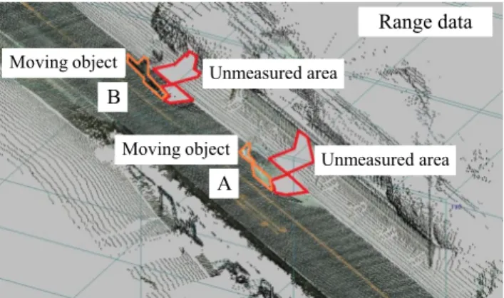
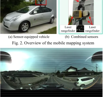
(2) Vision sensor. Laser rangefinder. (a) Sensor-equipped vehicle. GPS antenna. Laser rangefinder. (b) Combined sensors. Fig. 2. Overview of the mobile mapping system. Fig. 3. Example of an omnidirectional image. moving objects using a voting-based approach with a partial image mosaic. One problem inherent to this method is that the capturing vehicle must drive several times along the same road. On the other hand, there are other approaches [11][12] that detect moving objects using a vision sensor and laser rangefinder mounted on a mobile robot. However, the purpose of these research efforts has been to track moving objects. In our approach, we use a mobile mapping system that combines a visual sensor, laser rangefinders, an RTK-GPS, a gyroscope, and wheel encoders. Using this system, our proposed method generates a 3D model instantly or after a few driving measurements. It should be noted that the number of images used in our method is small compared with that required in a spatiotemporal image analysis. The rest of this paper is organized as follows. Section 2 describes the system used for our proposed method. Next, Section 3 describes the proposed method itself, and Section 4 presents our experimental results. Finally, Section 5 provides some concluding remarks regarding our proposal. 2. MOBILE MAPPING SYSTEM In this section, we describe the outline of our mobile mapping system, which was developed by Topcon Corporation. Fig.2 shows an overview of this system, which includes a visual sensor, laser rangefinders, an RTK-GPS, a gyroscope, and wheel encoders. Except for the wheel encoder, all sensors are mounted on the roof of the vehicle. The vision sensor used is a Ladybug3 omnidirectional sensor (Point Grey Research, Inc.), and has six cameras enabling the system to collect images from more than 80%. Point ｐ. S(ｐn-２) ｐn-２ Frame n-2. S(ｐn-1) ｐn-1 Frame n-1. S(ｐn) ｐn Frame n. S(ｐn＋1) ｐn＋1. S(ｐn＋２) ｐn＋２. Frame n+1. Frame n+2. Fig. 4. Relationship between 3D points and their projected points on omnidirectional images. of a full 360° view. The LMS291 laser rangefinder (SICK AG) collects 1D range data. As shown in Fig.2(b), the system has three laser rangefinders. One measures the distance of objects obliquely downward and behind the vehicle. The other two measure the distance of objects on the left and right sides of the vehicle, respectively, in a vertical direction. As the vehicle moves, the system can measure the surrounding environment. The location and position of the system are estimated using the RTK-GPS, gyroscope, and wheel encoders. Fig.3 shows an example of an omnidirectional image taken around position A from Fig.1. A moving object was photographed and can be seen on the right side of Fig.3. We detect the 3D points on moving objects from point cloud data using omnidirectional images, as described later. 3. DETECTION OF 3D POINTS ON MOVING OBJECTS In this section, we describe the method for detecting 3D points on moving objects from point cloud data. First, 3D points obtained by laser rangefinders are projected onto omnidirectional images. Under the assumption that the color of a pixel on the projected position of a static object is invariant to the viewing direction, we detect the points on a moving object using photometric consistency. The 3D points on moving objects are then detected using prior information on the road environment. 3.1. Detection using photometric consistency Fig.4 shows the relationship between 3D points and their projected points on omnidirectional images. Frame n is the nearest frame when the 3D point p is measured. This frame is referred to as a target frame, and we select 2M 1 frames including this target frame. We calculate the projection point on each image from the 3D point, and obtain the pixel values at this projected point. While each pixel value obtained from an omnidirectional image is value of 256 gradations for each RGB, we use the value based on the HSV model. In Fig.4 (for the case of M=2), the pixel values are represented by the S values of the HSV model. Similarly, the pixel values are also represented by the V values of the.

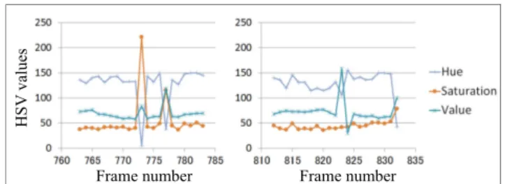
(3) 1 , ,. 2. 1 1. , ,. 2. 1. (1). ,. (2). This number is used to reduce the false detections from occlusions. The evaluation formula used for determining a point on a moving object is as follows.. ,. min min. , ,. , , . , ,. Frame number. at each point on. 2M 1 frames, and is the average of . In addition, k is the number of shifts from the target frame.. ,. Frame number. Fig. 5. HSV values on projected position of 3D points measured on moving red (left) and white (right) cars. is the average of. where. ,. HSV values. HSV model. We then calculate the variance of these values through the following equation.. ,⋯, ,⋯,. , , , ,. , , , ,. , ,. (3) (4). ,. ,. ,. (5). . where min{} is used to calculate the minimum value. The threshold Isth is determined through a discriminant analysis [13] using the evaluation value , for the 3D point of the same target frame. Similarly, the threshold Ivth is also determined through a discriminant analysis using the evaluation value , . When the evaluation value is either greater than or equal to the respective threshold, we determine that the point is located on a moving object. 3.2. Detection using prior information of the road environment To minimize the effect of detection errors, we select 3D points inside regions where moving objects existed on the road. More concretely, we calculate the horizontal distance between the system and point on the moving object, and then compute the histogram of the distance. When performing this calculation, the points corresponding to the road surface are excluded. If a peak exists in this histogram, it can be considered to be this side surface of the moving object. We then determine the length of this surface in the horizontal direction. On the other hand, the width of the moving object traveling on a road is roughly known. We search the points on moving objects in the height direction within the range of its length and known width, and detect the highest point. Through the above process, we can determine the rectangular solid where the moving objects existed on the road. In addition, to decrease detection errors, it is necessary to select a slightly larger range in this space.. 4. EXPERIMENTAL RESULTS To verify the effectiveness of the proposed method, we measured outdoor environments using the described system, and tested the proposed method using measured point cloud data. The image data from the test dataset used were taken at every 4 m, and measurement cycle of the laser rangefinder was 75 Hz. A total of 25,000 points were used in this experiment. In order to verify the effectiveness of the photo consistency based moving object detection, we first observed the change of the HSV values of two different 3D points measured on moving objects of different colors (Fig.5). In this figure, moving red and white cars are measured in the 773rd-frame and the 823rd-frame, respectively. From these results, we can see that changes of the H, S, V values depend on the color of moving objects, and that the observation of the photo consistency for each H, S, V component alone is not sufficient for our purpose. Fig.6 shows an image synthesized from the original omnidirectional image and the measurement results of the laser rangefinder. The 25,000 points are projected onto the omnidirectional image by utilizing data from the RTK-GPS, gyroscope, and wheel encoders. These projected points can be found by comparing Figs. 3 and 6. The projected points are indicated by the white and gray dots, and are based on the results of Eq. (5). The white dots indicate the points located on moving objects, whereas the gray dots indicate the points located on stationary objects. We used M=2 in this experiment to determine the evaluation value. Fig.7 shows a histogram representing the distribution of horizontal distances between the measurement system and points on a moving object. It should be noted that a positive number on the horizontal axis indicates the right side of the system, and a negative number represents the left side. The results in Fig.7 exclude 3D points on the road surface. A peak at a distance of 2.2 m can be seen in this histogram. Next, we choose a rectangular solid based on this peak and detect the points on the moving objects. We assumed that the width of a moving object is 2 m, and to avoid any missed detections, we used a rectangular solid 30 cm larger than the rectangular solid obtained above. Fig.8 shows the final detection results. The white dots indicate the points on moving objects, and the gray dots are the points on stationary objects. Table 1 shows the percentage of points.

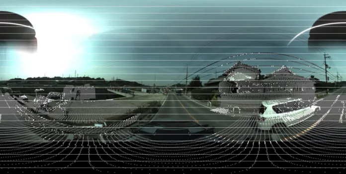
(4) Fig. 6. Image synthesized from the original omnidirectional image and the measurement results of the laser rangefinder. Frequency. Table 1 Detection Result. Distance (m) Fig. 7. Horizontal distances between the measurement system and points on a moving object (excluding the road surface). Without prior information. Final results. Detection rate (%). 62.5. 94.8. Miss rate (%). 37.5. 5.2. False detection rate (%). 7.1. 0.0. percentage of erroneously detected points on a stationary object. Table 1 shows the results from before and after information on the road environment is used. In this experiment, the final detection rate was 94.8% and the final false rate was 0.0%. From these results, it can be confirmed that points on the moving objects were properly detected by our proposed method. 5. CONCLUSIONS In this paper, we proposed a method for detecting 3D points on moving objects from 3D point cloud data based on photometric consistency and prior information of the road environment. We confirmed experimentally the effectiveness of the proposed method. Future work will be conducted to interpolate missing 3D points caused by occlusions from moving objects. ACKNOWLEDGEMENT. Fig. 8. Final detection result using the proposed method. detected on moving objects. The detection rate indicates the percentage of points correctly detected on a moving object. The miss rate is the percentage of points missed on a moving object. The false detection rate indicates the. This work was partially supported by Grant-in Aid for Scientific Research Nos. 23240024 and 24500234 from the Ministry of Education, Culture, Sports, Science and Technology..

(5) REFERENCES [1] S. Agarwal, N. Snavely, I. Simon, S. M. Seitz, and R. Szeliski, “Building Rome in a Day,” in ICCV, pp.72-79, 2009. [2] Y. Furukawa, B. Curless, S.M. Seitz, and R. Szeliski, “Towards Internet-scale Multi-view Stereo,” in CVPR, pp. 1434-1441, 2010. [3] T. Sato, H. Koshizawa, and N. Yokoya, “Omni directional Free-viewpoint Rendering Using a Deformable 3-D Mesh Model,” Int. Journal of Virtual Reality, Vol.9, No.1, pp.37-44, 2010. [4] S.F. El-Hakim, C. Brenner, and G. Roth, “A Multi-sensor Approach to Creating Accurate Virtual Environments,” Jour. of Photogrammetry & Remote Sensing, Vol.53, pp.379-391, 1998. [5] H. Zhao, and R. Shibasaki, “Reconstruction of Textured Urban 3D Model by Fusing Ground-Based Laser Range and CCD Images,” IEICE Trans. Inf. & Syst., Vol.E-83-D, No.7, pp.14291440, 2000. [6] C. Früh, and A. Zakhor, “An Automated Method for LargeScale, Ground-Based City Model Acquisition,” Int. Jour. of Computer Vision, Vol.60, pp.5-24, 2004. [7] A. Banno, and K. Ikeuchi, “Shape Recovery of 3D Data Obtained from a Moving Range Sensor by using Image Sequence,” in ICCV, Vol.1, pp.792-799, 2005.. [8] T. Asai, M. Kanbara, and N. Yokoya, “Data Acquiring Support System Using Recommendation Degree Map for 3D Outdoor Modeling,” Proc. SPIE Electronic Imaging, Vol.6491, pp.6491064910H-8, 2007. [9] G. Petrie, “Mobile Mapping Systems: An Introduction to the Technology,” GEOInformatics, Vol.13, pp.32-43, Jan./Feb. 2010. [10] H. Uchiyama, D. Deguchi, T. Takahashi, I. Ide, and H. Murase, “Removal of Moving Objects from a Street-View Image by Fusing Multiple Image Sequences,” in ICPR, pp.3456-3459, 2010. [11] B. Jung, and G.S. Sukhatme, “Detecting Moving Objects using a Single Camera on a Mobile Robot in an Outdoor Environment,” in International Conference on Intelligent Autonomous Systems, pp.980-987, 2004. [12] B. Jung, and G.S. Sukhatme, “Real-time Motion Tracking from a Mobile Robot,” in International Journal of Social Robotics, Vol.2, No.1, pp.63-78, 2010. [13] N. Otsu, “A Threshold Selection Method from Gray Level Histograms,” IEEE Trans. Systems, Man and Cybernetics, Vol.9, pp.62-66, 1979..

(6)