A Depth First Search Algorithm for Optimal Triangulation　of Bayesian 　Networks

(1)

深さ優先探索を用いたベイジアンネットワークの最適三角化

A Depth First Search Algorithm for Optimal Triangulation of

Bayesian Networks

李超

1∗

_{植野真臣}

1

Chao Li

1

Maomi Ueno

1

_{電気通信大学大学院情報システム学研究科}

1

_{Graduate School of Information Systems, The University of Electro-Communications}

Abstract: The most popular algorithm for exact inference on Bayesian networks is the

junc-tion tree propagajunc-tion algorithm. To improve the time and space complexity of the juncjunc-tion tree algorithm, we must find an optimal triangulation. For this purpose, Ottosen and Vomlel have pro-posed a depth-first search (DFS) algorithm for optimal triangulation using branch-and-bound and dynamic clique maintenance techniques. Nevertheless, their method entails heavy computational costs. To mitigate this problem, we propose an extended depth-first search (EDFS) algorithm. The new algorithm EDFS improves the DFS algorithm in the following two ways: (1) reduction of the computational cost of each lower bound calculation, and (2) reduction of the branching factor of each node expansion. Experimental results show that the proposed method is markedly faster than the Ottosen and Vomlel method.

1 Introduction

In the junction tree algorithm, a Bayesian network is first converted into a special data structure called a junction tree; then belief is propagated on that tree. A junction tree can be formed if and only if the under-lying graph of the Bayesian network is triangulated. If the graph is not triangulated, then we must add extra edges to it until it becomes so. Although trian-gulation does not change any accuracy of belief prop-agation, it improves the time and space complexity of the junction tree algorithm. As described in this pa-per, we specifically examine the discovery of an opti-mal triangulation. Unfortunately, finding an optiopti-mal triangulation is NP-hard [1]. However, this defect is not crucially important because the triangulation can often be done off-line and can be saved for inference algorithms.

Previous investigations of triangulation problems have been conducted by researchers from various fields for different purposes. These triangulation algorithms are designed to optimize criteria of various kinds. The commonly used criteria are the fill-in, the treewidth,

∗_{連絡先：電気通信大学大学院情報システム学研究科}

〒 182-8585 東京都調布市調布ヶ丘 1-5-1 E-mail: [email protected]

E-mail: [email protected]

and the total table size. Of all commonly used op-timality criteria, the total table size criterion yields the most exact bounds of the memory and time re-quirements of probabilistic inference. As described in this paper, we consider the problem of ascertaining an optimal total table size triangulation of Bayesian net-works. We solve this problem by searching the space of all possible triangulations. This search is conducted by enumerating all possible elimination orders and for choosing one of those that have the minimum total ta-ble size.

To obtain an optimal triangulation for total table size criterion, Ottosen and Vomlel investigated depth-first search and best-depth-first search algorithms [2]. They claimed that the depth-first search uses less mem-ory than the best-first search does. Moreover, they demonstrated that the two methods have almost equal run time in computational experiments. The best-first search with theoretically better order does not necessarily run faster than the depth-first search in practice. Although the depth-first search expand more search nodes than the first search does, the best-first search has heavy overhead costs for maintaining a priority queue. For the optimal triangulation algo-rithm, it is important to make the overhead as low as possible when reducing the search space.

Further-人工知能学会研究会資料 SIG-FPAI-B403-05

(2)

more, Ottosen and Vomlel improved the naive depth-ﬁrst search by introducing the eﬃcient dynamic main-tenance of the cliques of a graph and coalescing map pruning techniques. However, the method still entails a heavy computational cost.

In this paper, we propose an extended depth-ﬁrst search algorithm for optimal triangulation of Bayesian network. The algorithm improves the Ottosen and Vomlel method as follows.

(1) It reduces the computational cost of each lower bound calculation.

(2)It reduces the branching factor of each node ex-pansion.

For 1, we propose a new dynamic clique mainte-nance algorithm that explores less search space and which runs faster than the Ottosen and Vomlel method does. The new dynamic clique algorithm can im-prove the computational cost that is inherent in cal-culation of the lower bound at each node. Thereby, the overhead decreases. For 2, we introduce a new pruning rule called pivot clique pruning. The prun-ing method cuts some search nodes without heavy computation. We show that the new pruning rule can reduce the search space considerably, whereas the overhead is still low because of the simplicity of the pruning method. Some simulation experiments show that the proposed algorithm combining these two im-provements is markedly faster than the Ottosen and Vomlel method.

2 Triangulation

This section deﬁnes notation used in the triangula-tion problem and then formulates the search space of the optimal triangulation algorithm.

2.1 Notation for triangulation

Let G = (V, E) be an undirected graph with vertex set V and edge set E. For a set of vertices W ⊆ V, G[W] = (W,{ (v, w) ∈ E | v, w ∈ W}) is the subgraph of G induced by W. For a set of edges F, all the end point vertices of edges in F { v,w | (v, w) ∈ F} are denoted byV(F).

Two vertices v and w are said to be adjacent if (v, w)∈ E. The neighbors N (v, G) of v ∈ V are the set of vertices that are adjacent to v. For a set of vertices W ⊆ V, N (W, G) denotes the (∪w∈WN (w, G))\W.

The family FA(W, G) of a set of vertices W is the set N (W, G)∪W.

Graph G is complete if all pairs of vertices{ u,v } (u̸= v) are adjacent in G. A set of vertices W ⊆ V is complete in G if G[W] is a complete graph. If W is a complete set and no complete set U exists such that W

⊂ U, then W is a clique.(Remark: Any complete set is

called a clique in some literatures. In that case, what we deﬁned as a clique is called a maximal clique.) The set of all cliques of graph G is denoted as C(G). The set of all cliques that intersect a set of vertices W is denoted as C(W, G). If G’ = (V, E∪F) ( F ∩ E= ∅) is the graph resulting from adding a set of new edges F to G = (V, E), thenRC(G,G’) = C(G) \ C(G’) is the set of removed cliques, and N C(G,G’) = C(G’)\

C(G) is the set of new cliques.

A chord of a cycle C is an edge not in C with end-points lying in C. A chord-less cycle in G is a cycle of length greater than three in G that has no chord. An undirected graph is triangulated (or chordal) if it has no chordless cycle. A triangulation of G is a set of edges T such that T ∩ E= ∅ and the graph H = (V,E ∪ T) is triangulated.

Vertex elimination algorithm is used to triangulate graphs. Elimination of a vertex v∈ V of G = (V, E) is the process of adding edges between every pair of the vertices inN (v, G), then removing v and all the incident edges from graph G. The added edges are called fill-in edges. This process induces a partially triangulated graph H = (V, E∪F), where F is fill-in edges, and the remafill-infill-ing graph is denoted by R = H[V/{v}]. If F = ∅, then v is called a simplicial vertex.

An elimination order of an undirected graph G = (V, E) is a bijection π : V → {1, 2, . . ., |V| } that speciﬁes a vertex ordering for eliminating all vertices V from G. Given any elimination order π, if all vertices are eliminated sequentially from G according to π, then the union of all the ﬁll-in edges is a triangulation of G.

The table size of a clique C is given as ts(C) = ∏

(v∈C)|sp(v)|, where sp(v) denotes the state space of

the variable corresponding to v in the Bayesian net-work. Finally, the total table size (TTS) of a graph H is given as tts(H)=∑_C_∈C(H)ts(C). Any

tion order π which can be used to direct an elimina-tion scheme and induce a triangulated graph H. The TTS of graph H is also called the TTS of π. Any elimination order π that induces a triangulation with minimum TTS is an optimal elimination order. The

(3)

triangulation corresponding to the order π is an opti-mal triangulation.

2.2 Search space of the optimal

trian-gulation algorithm

We conduct a search in the space of all possible elimination orders of the moralized graph of Bayesian network to ﬁnd the optimal triangulation[2]. To do so, we generate a search graph that includes all elimina-tion orders. The search graph is a tree with leaf nodes corresponding to distinct elimination order. (In this paper, the term “node” is used exclusively for a point in the search space. The term “vertex” is used ex-clusively for a point in the graph being triangulated). We eliminate one vertex at each node expansion step and associate the node with an induced intermedi-ate partially triangulintermedi-ated graph. In this search space, each node is labeled using a partial elimination order

τ . Each child of a node is generated by eliminating

a vertex from the parent’s remaining graph and ap-pending the vertex to the parent’s partial order. For the root nodes where we start the search, no vertex has been eliminated. For the leaf nodes, all vertices have been eliminated. The associating graph has been triangulated.

3 The Ottosen and Vomlel

algo-rithm

This section presents a review the depth-ﬁrst search algorithm with upper bound pruning presented by Ot-tosen and Vomlel [2].

3.1 Upper Bound

The naive depth-first branch and bound algorithm operates as follows. We maintain a global variable upper bound (UB) to store the optimal TTS triangu-lation found to date. First, we initialize UB with the triangulation using minimum fill-in heuristic, which greedily selects the next vertex to eliminate if the ver-tex leads to add the minimum fill-in edges. Next, it traverses all search tree nodes in a depth-first man-ner. We calculate the TTS of each node, which is a lower bound of the node. If we find a node of which the lower bound on TTS is greater than UB, then we prune all the successors from the node. However, if

1:procedure CliqueUpdate(G, C, tts, F) 2: Let G’=(V,E∪F) 3: Let U =V(F) 4: for all C∈ C do 5: if C∩ U ̸= ∅ then 6: SetC = C \ {C}

7: let Cnew = BKalgorithm(G’[FA(U, G’)])

8: for all C∈ Cnew do

9: if C∩ U ̸= ∅ then

10: SetC = C ∪ {C}

図 1: Maintenance of cliques by local search. we ﬁnd a complete ordering that is better than UB, we update the UB. When the search terminates, the ﬁnal UB is reported as the optimal triangulation.

3.2 Lower Bound

We want to use the TTS upper bound for pruning branches in depth-ﬁrst search triangulations. There-fore, we must also associate the TTS lower bound with each node in a search tree. On each node expansion step, the total table size of the induced partially tri-angulated graph is a lower bound because adding an edge to graph G cannot decrease the total table size [2]. The total table size is easy to compute if we know the cliques of the partially triangulated graph. There-fore, we must also associate the set of cliques with each node. In Ottosen and Vomlel[2], for computing the lower bound(TTS), each node t is represented as a tuple (τ ,H,C,tts).

t.τ : a list of vertices representing the partial elimi-nation order.

t.H = (V,E∪F): Original graph with all ﬁll-in edges F accumulated along the τ .

t.C: A set of cliques for H, C(H).

t.tts: Total table size of graph H, which is a lower bound for node t.

To compute t.tts, we must calculate all the cliques

t.C ﬁrst. For this purpose, we can use a standard

clique enumeration algorithm such as the well-known Bron–Kerbosch algorithm (BK algorithm) [3]. How-ever, the BK algorithm engenders many redundant computations. Ottosen and Vomlel [2] proposed a more eﬃcient algorithm for computation of the set of cliques C in a dynamic graph. We explain the dy-namic clique maintenance algorithm in section 3.3.

3.3 Dynamic clique maintenance

Ottosen and Vomlel [2] pointed out that recomput-ing all cliques is unnecessary. They proposed the fol-lowing dynamic clique maintenance algorithm. The

(4)

main idea behind the algorithm is simple. Instead of searching for all cliques in the whole graph, as the BK algorithm does, their algorithm runs a clique enu-meration algorithm simply on a smaller subgraph on which all the new cliques appear and on which the existing cliques on the subgraph disappear. This dy-namic clique maintenance algorithm is presented in Fig. 1, where G is the initial graph, C stands for the set of cliques in G, tts denotes the total table size of G, F signiﬁes the ﬁll-in edges, and G’ is derived by adding F to G. BKalgorithm(G) returns a set of cliques of the graph G. The algorithm is derived based on the following theorem:

Theorem 1 (Ottosen and Vomlel [2]) Let G = (V,

E) be an undirected graph, and let G’ = (V, E∪ F) be the graph resulting from adding a set of new edges F to G. Let U =V(F). The clique set C(G’) can be found by removing the cliques ofC(U,G) and by adding cliques of C(U,FA(U, G’)])

we ﬁnd that the algorithm sometimes removes and adds the same cliques again. Although Ottosen’s ap-proach reduces the search range of the expensive enu-meration algorithm BKalgorithm(G) to a small sub-graph, the method might present shortcomings in per-formance as the number of duplicated cliques becomes large.

3.4 Depth-First Search for optimal

tri-angulation

We explained the search tree of depth-first search and how to compute a lower bound efficiently for each node. The depth-first search algorithm presented by Ottosen and Vomlel can be implemented in O(|V|) space and O(|V|!) time. In order to prune unnec-essary search processes further, Ottosen and Vom-lel also introduced the following pruning rules: (1) Graph reduction techniques called the simplicial ver-tex rule, and (2) pruning based on a coalescing map. The complete algorithm of the Ottosen and Vomlel approach is shown in Fig. 2. The procedure Elimi-nateVertex(m,v) simply eliminates a vertex from the remaining graph R and updates the cliques and TTS of the partially triangulated graph. The procedure EliminateSimplicial(m,v) removes all simplicial ver-tices from the remaining graph. Although it is known that the depth-first search runs in O(|V|!), the algo-rithm combined with the techniques described above

1:function TriangulationByDFS(G)

2: Let s = (G,C(G),tts(G),V)

3: EliminateSimplicial(s)

4: if|V(s.R)|=0 then

5: return s

6: Let best = MinFill(s) ▷ upper bound

7: Let map =∅ ▷ Coalescing map

8: ExpandNode(s,best,map) return best

9:procedure ExpandNode(n,&best,&map) 10: for all v∈ V(n.R) do 11: Let m = Copy(n) 12: EliminateVertex(m, v) 13: EliminateSimplicial(m) 14: if|V(m.R)|=0 then 15: if m.tts<best.tts then 16: Set best = m 17: else 18: if m.tts≥best.tts then

19: continue ▷ upper bound pruning

20: if map[m.R].tts≤m.tts then

21: continue ▷ node Coalescing

22: Set map[m.R] = m

23: ExpandNode(m,best,map)

図 2: Depth-ﬁrst search with coalescing and upper-bound pruning. 1:procedure newCliqueUpdate(G, C, tts, F) 2: Let G’=(V,E∪F) 3: Let U =V(F) 4: for all C∈ C(G) do 5: if C⊆ W then 6: SetC = C \C

7: let Cnew = BKalgorithm(G[W])

8: for all C∈ Cnew do

9: SetC = C ∪ C

図 3: Maintenance of cliques by reduced local search. merely hits the upper bound. Ottosen and Vomlel [2] claimed that their algorithm actually runs in O(2|V |) time in practice. Nevertheless, their method still en-tails a heavy computational cost. We therefore pro-pose the following new algorithm to overcome this problem.

4 New algorithm

4.1 New dynamic clique maintenance

In the depth-ﬁrst search triangulation algorithm, we must compute the TTS of a search node. For this purpose, we must update cliques of the partially tri-angulated graph eﬃciently. In section 3.3, we have demonstrated that the Ottosen and Vomlel approach might have the duplicated clique problem. To solve this problem, we propose a new algorithm. The new dynamic clique maintenance algorithm is based on the following Theorem:

Theorem 2 Let G = (V, E) be an undirected graph,

and let G’ = (V, E ∪ F) be the graph resulting from adding a set of new edges F to G. Let U =V(F) and W = { u | (v, w) ∈ F and v, w ∈ N (u,G’)} ∪ U. The

(5)

C(G’) can be found by removing the cliques C ⊆ W; and then by adding cliques ofC(G’[W]).

The new dynamic clique maintenance algorithm per-forms BK algorithm on W, which is a subgraph of G’[FA(U, G’)] on which the Ottosen and Vomlel method does. The clique enumeration algorithm (BK algo-rithm) entails exponential costs with number of ver-tices. Therefore, the reduction of the search graph size is eﬀective to reduce the calculation costs. The proposed algorithm is shown in Fig 3.

4.2 Pivot clique pruning

1:Insert lines 1–10 of Algorithm in Fig. 2

2:procedure ExpandNode(n,&best,&map)

3: for all v∈ V(n.R)\SelectOneClique(n.H) do

4: Let m = Copy(n)

5: EliminateVertex(m,v)

6: EliminateSimplicial(m)

7: Insert lines 16–29 of Algorithm in Fig. 2

図 4: Depth-ﬁrst search with pivot node pruning. In this section, we propose the pivot clique pruning. In the Ottosen and Vomlel depth-ﬁrst search triangu-lation algorithm, we generated a successor node for each vertex in the remaining graph R. Indeed, it is possible to reduce some successors based on the fol-lowing theorem.

Theorem 3 Let G be an incomplete graph with at

least three vertices. Suppose that we eliminate a graph G along the partial elimination order τ = { v1, v2, . . ., vi−1}. Now, The partially triangulated graph is

H, and the remaining graph is R. We can choose any clique Cpivot in H as pivot clique. Rather than

gen-erated a successor search node for each vertex in the remaining graph R, the depth-first search can safely remove all the successors that corresponds to the ver-tices in the Cpivot.

This theorem is applicable to pruning some branches with the depth-ﬁrst search algorithm. The pruning is that we choose a clique Cpivot from the clique set of

the search node, we prune the successor nodes for the vertices in Cpivot. The Cpivot is called pivot clique.

We describe the algorithm with pivot clique pruning in Fig 4. In the algorithm line 3, we generate search nodes for the vertices inV(n.R)\SelectOneClique(n.H). The procedure SelectOneClique(G) simply iterates all the cliques corresponding to the node and choose the clique which has the largest intersection with remain-ing graph R. The search tree size can be reduced from

|V|! to O(|V-2|!), Since a clique has at least two

ver-tices, we can omit at least two branches in each node expansion.

5 Experiments

We conduct computational experiments to demon-strate the advantages of our proposed method over the Ottosen and Vomlel method.

5.1 Dynamic clique maintenance

図 5: Comparison of the running times of the l method and the proposed method for dynamic clique mainte-nance.

In this section, we compare the proposed method for dynamic clique maintenance and the Ottosen and Vomlel method. For that purpose, we used a set of public Bayesian networks 1 _{. We also generated 300}

random Bayesian networks with size 30 using BN-Generator2. Then we performed the following test on the two data sets: For each graph in the datasets, triangulate the graph by vertex elimination algorithm in some random order. The set of cliques is updated after each vertex is eliminated. This test will show the expected speedup of our proposed method for triangulation problem. For each graph, we sequen-tially eliminate all vertex to triangulate the graph 10000 times(with diﬀerent random order on each run). For each public Bayesian network, we report the to-tal time (10000 times triangulation) of our proposed method and the Ottosen and Vomlel method in Ta-ble 1. Fig. 5 shows the running time of proposed algorithm divided by the time of Ottosen’s algorithm

1_{http://www.cs.huji.ac.il/site/labs/compbio/Repository/} 2_{http://sites.poli.usp.br/pmr/ltd/Software/BNGenerator/}

(6)

表 1: Running time results for real-world Bayesian networks.

Bayesian Networks CPU time (seconds)

name V E Proposed Ottosen and Vomlel Ottosen and Vomlel/Proposed child 20 30 0.32186 0.77234 2.39951 insurance 27 70 0.65473 1.78803 2.73090 water 32 123 1.29116 3.37409 2.61321 mildew 35 80 0.69941 2.48839 3.55782 alarm 37 65 0.68804 1.93631 2.81420 barley 48 126 1.43195 5.57423 3.89274 hailfinder 56 99 1.47428 4.93131 3.34488 win95pts 76 225 3.45127 12.2935 3.56204

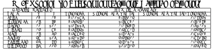
表 2: A comparison of the depth-ﬁrst search triangulation algorithms with various dynamic clique maintenance procedure and the proposed triangulation algorithm.

Bayesian Networks DFS DFS-D DFS-P EDFS

name V Time(s) Branches Nodes Time(s) Branches Nodes Time(s) Branches Nodes Time(s) Branches Nodes Insurance 27 1.656 4818 2291 0.776 4818 2291 0.944 3251 1736 0.358 3096 1919 Water 32 10.415 14438 6816 4.767 14438 6816 7.81 13551 6191 1.311 8049 5187 Mildew 35 13.285 69310 22351 5.246 69310 22351 6.317 38204 14741 0.803 15349 5222 Alarm 37 0.013 35 27 0.006 35 27 0.005 26 24 0.005 27 25 Hailfinder 56 8.869 44270 19650 4.337 44270 19650 4.847 44657 17052 2.126 31289 12537 WIN95PTS 76 60.082 74227 34993 27.146 74227 34993 21.094 46679 22426 6.922 32084 14669

for all random Bayesian networks. The result for 300 random Bayesian networks on Fig. 5 shows that our proposed algorithm is constantly and in average 2.37 times faster than the Ottosen and Vomlel approach.

5.2 Optimal triangulation

In this section, we describe the experimental results for optimal triangulation algorithm for total table size criteria. For examine the eﬀectiveness of each pro-posed method given in Section 5, we give names for intermediate algorithms as follows.

DFS: Ottosen and Vomlel depth-ﬁrst search opti-mal triangulation algorithm

DFS-D: improved DFS obtained by introducing only the technique in section 5.1.

DFS-P: improved DFS obtained by introducing only the technique in section 5.2.

EDFS: improved DFS obtained by introducing the combination of the techniques in section 5.1 and 5.2. We used six well-known graphs in the Bayesian net-work repository. The results are presented in Table.2. The Branches count the number of nodes has been expanded. The Nodes means the size of the coalesc-ing map, which is the most memory consumcoalesc-ing data structure used in the depth-ﬁrst search triangulation algorithm. The experiment results show that our al-gorithm (EDFS) is 4-20 times faster than DFS in some cases, and pivot clique pruning lead to a signiﬁcant memory reduction. From the result in Table.2, we no-ticed that branches of DFS-P is about half of branches of DFS. In section 5.2, we had gave the theoretical re-sult that search tree size can be reduced from |V|! to |V-2|!, but the upper bound in practice rarely be

touched. From our experiment, the pivot clique prun-ing reduces the search space size to the half size.

6 Conclusions

We proposed a depth-ﬁrst search algorithm for op-timal triangulation of Bayesian networks. Our algo-rithm retains the simplicity of the Ottosen and Vomlel algorithm while reducing the search space quite eﬃ-ciently with low overhead.

As a subject for future work, we intend to investi-gate heuristic triangulation algorithms for on-line pur-poses. We shall also investigate a new graph search reduction method to improve the search space of the optimal triangulation algorithm.

参考文献

[1] Wilson X. Wen: Optimal decomposition of belief net-works, Proceeding UAI ’90 Proceedings of the Sixth

Annual Conference on Uncertainty in Artificial In-telligence, Pages 209 - 224, (1990)

[2] Thorsten Jorgen Ottosen, Jiri Vomlel: All Roads Lead To Rome–New Search Methods for Optimal,

International Journal of Approximate Reasoning,

vol.53, no.9, pp.1350–1366, 2012.

[3] Thorsten Jorgen Ottosen, Jiri Vomlel: All Roads Lead To Rome–New Search Methods for Optimal,

International Journal of Approximate Reasoning,

A Depth First Search Algorithm for Optimal Triangulation of Bayesian Networks

深さ優先探索を用いたベイジアンネットワークの最適三角化