Shrinking population and the urban hierarchy
著者
Kim Ho Yeon
権利
Copyrights 日本貿易振興機構(ジェトロ)アジア
経済研究所 / Institute of Developing
Economies, Japan External Trade Organization
(IDE-JETRO) http://www.ide.go.jp
journal or
publication title
IDE Discussion Paper
volume
360
year
2012-08-01
i
INSTITUTE OF DEVELOPING ECONOMIES
IDE Discussion Papers are preliminary materials circulated to stimulate discussions and critical comments
Keywords: Population shrinkage, Rank-size rule, Central place theory JEL classification: R12, R23
* Professor, Dept. of Economics, Sungkyunkwan University ([email protected]). The author stayed at IDE from July 29, 2011 to January 28, 2012 as a Visiting Research Fellow (VRF). This paper is based on the research during the period and comprises a part of the results of VRF Program (VRF Series No.474).
IDE DISCUSSION PAPER No. 360
Shrinking Population and the
Urban Hierarchy
Ho Yeon KIM*
August 2012
Abstract
This paper examines whether population shrinkage leads to changes in urban hierarchy in terms of their relative size and function from the standpoint of the new economic geography. We find some salient patterns in which small cities in the agglomeration shadow become relatively bigger as medium industries spill over on them. This appears to be quite robust against a variation in the rate of natural change among cities. Thus, rank-size relationship and the urban hierarchy are partly disrupted as population shrinks. Regarding the welfare of the residents, a lower demand for land initially causes rent to go down, which boosts the utility. However, the illusion is short-lived because markets soon begin to shrink and suppress wages. We also find that it is better to maintain a slow pace of overall population decline in the long-term perspective. More importantly, it is crucial to sustain the relative livability of smaller cities to minimize the overall loss of utility.
ii
The Institute of Developing Economies (IDE) is a semigovernmental, nonpartisan, nonprofit research institute, founded in 1958. The Institute
merged with the Japan External Trade Organization (JETRO) on July 1, 1998.
The Institute conducts basic and comprehensive studies on economic and related affairs in all developing countries and regions, including Asia, the Middle East, Africa, Latin America, Oceania, and Eastern Europe.
The views expressed in this publication are those of the author(s). Publication does not imply endorsement by the Institute of Developing Economies of any of the views expressed within.
INSTITUTE OF DEVELOPING ECONOMIES (IDE), JETRO 3-2-2, WAKABA,MIHAMA-KU,CHIBA-SHI
CHIBA 261-8545, JAPAN
©2012 by Institute of Developing Economies, JETRO
No part of this publication may be reproduced without the prior permission of the IDE-JETRO.
1
1. Introduction
The population of Korea is expected to dwindle starting around 2030. In addition to a loss of economic vitality, the shrinking population would bring about a shortage of workforce and manpower as well as a skewed demography, resulting in low self-confidence and an overall reduced productivity. Also, the rising cost of care for the elderly and lower rates of investment from firms would deteriorate the quality of life in general. Its impact on the urban hierarchy of Korea is of particular interest. The Seoul National Capital Area occupies only 11.8% of the entire land, yet it accommodates 24.5 million inhabitants, almost half of the country’s population. Understandably, the Korean government has been obsessed with the idea of a decentralization of industry and a balanced growth of regions. Through myriads of laws and regulations, the central authority tried hard to drive out firms and people by inducing them to non-capital areas with favorable environments.
Other smaller cities are worth looking into. Busan is Korea’s second largest metropolis, with a population of around 3.5 million. It is the largest port city in Korea and the fifth busiest seaport in the world. Incheon became important because of its location which made it a good harbor; when the port was founded in 1883, the city had a population of only 4,700. Incheon is now home to over 2.5 million people. Daegu is the city of the manufacturing industry. Remarkable manufacturing factories such as Samsung are located near the city. Being known as the Silicon Valley of Korea, Daejeon is home to various private and public research institutes, centers and science parks. The mutual stimulation and cooperation between these communities produce remarkable innovation and commercialization of technologies. Ulsan is the industrial powerhouse, which is home to the world’s largest automobile assembly plant, shipyard and oil refinery. In 2008, Ulsan had a GDP per capita of $63,817, the highest by far in Korea. Although these cities seem to be thriving for now, it is quite uncertain how they would fare in an era of diminishing population and expectations.
There have been many regional development polices since the 1970s, an era of fast growth. One important aspect that has been found consistently in these policies is that they all aimed for regional equity; regional development policy meant a balanced regional development policy in Korea. Regional disparity was discussed in the framework of capital vs. non-capital areas, and many measures were taken to reduce the gap. Such measures include constructing SOC in underdeveloped regions, providing incentives for firms in the capital area to relocate to non-capital regions, building up and subsidizing industry bases in underdeveloped regions, controlling the expansion of the capital area, and so on. Thus, Korea’s regional development policy is synonymous with the growth management of SNCA.
This study aims at eliciting the consequences of an impending population shrinkage on the social and economic aspects of an economy, especially a systematic analysis of its spatial implication. Given a huge concentration of population in the capital area, it would be a meaningful task to investigate the potential outcome of a decreasing population in the city systems of Korea or any other country facing a similar problem.
Previous literature is generally silent about the effects of a negative external shock in terms of population. It is uncertain, for example, whether there would be a system wide reduction of population across the board or a disappearance of smaller cities with primary city becoming larger, or vice versa. In any case, the underlying mechanism of agglomeration, as empirically identified by Rosenthal and Strange (2001), would now start working backwards so that all knowledge spillovers, labor market pooling, and input sharing are reduced. The remainder of this paper is organized as follows. The next section discusses the recent phenomena of population shrinkage. Section 3 reviews the related literature. Section 4 describes the model structure. Section 5 presents the simulation results, and section 6 concludes the paper.
2
2. Population shrinkage
According to the United Nations, the world population reached 7 billion in October 2011, and they estimate that there will be 9.3 billion by 2050. As a baby boom generation enters the labor force, a country can enjoy a demographic dividend with a rising income and a low dependency ratio. As that generation retires, however, the dividend turns to a liability with population growth stagnant or falling.
Figure 1 illustrates total fertility by major regions. The fertility rate is the number of children an average woman is likely to have during her childbearing years of 15-49. In general, 2.1 is considered the replacement level of fertility, allowing for early mortality. By 2020, the global fertility rate will dip below the global replacement rate for the first time. The world’s population will stabilize at 9.2 billion in 2050. Wealth and fertility go together negatively. Low fertility enables rapid accumulation of capital per head. A shortage of workers, however, eventually pushes up wage costs.
Figure 2 shows the population figures for Japan and Korea. Japan, once called the lead goose, is now the oldest goose. Japan is the fastest aging society and the first big country in history to have started shrinking rapidly from natural causes. In the 2005 census, the number of deaths exceeded that of births for the first time. The working age population hit its highest point in 1995, and by 2050 it will be smaller than it was in 1950. Employment rates among women have increased, and private companies discourage mothers from returning to their old jobs.1 What took place in Britain over 130 years (1800-1930) took place in Korea over just 20 years (1965-1985).2
Women get married later or don’t get married at all. Marriages are also breaking down, which is a recent change in Asia. Some blame the improvements in women’s education and income. In Korea women earn half of all the master’s degrees. More education leaves the best-educated women with fewer potential partners. In Korea the employment rate of women in their 20s (59.2%) overtook that of men (58.5%). The collapse of lifetime employment systems in Japan and Korea means that the wife’s earnings are needed. They put off having children while they pursue a career. They are faced with an unwelcomed choice between a career and a family. The best-educated and highest-paid women face great opportunity cost of having children. Park (2006) surmised that the high costs of education for children and the increasing labor participation of women were decisive in lowering the fertility rate of Korean women. In China, 118 boys were born to every 100 girls due to sex-selective abortions. In 2030 about 8% of Chinese men aged 25 and older will be unable to marry.
The total fertility rate of Korea was at a record low of 1.15 in 2009, the lowest in OECD countries and well below the replacement level.
3
What would happen to cities when their population implodes? According to Nakajima (2008), the separation of Japan and Korea brought a negative effect, more so on smaller cities than on larger cities. Border cities in Japan suffered a greater decline due to the loss of accessibility to the colonial markets, causing a subsequent relocation of industry and people. From a theoretical standpoint, Holmes (1999) explained that in the standard economic geography model, the equilibrium output of a particular variant is independent of population. When the elasticity of substitution is low, as population increases, total local production expands not only by adding new varieties but also by increasing the output of existing products. Thus, there might be a convex relationship between local production and population.
1
“Into the unknown: A special report on Japan”, The Economist, November 20, 2010.
2
“Go forth and multiply a lot less”, The Economist, October 31, 2009.
3
3
3. Review of the Literature
What happens to an urban system when its population decreases is not so well documented. An insight to this question can be gained from Fujita et al. (1999). Given that the cities within an economy constitute some form of hierarchical structure, they model the endogenous formation of a hierarchical urban system. To overcome the multiplicity of equilibria, they propose an evolutionary approach which combines a general equilibrium model with an adjustment dynamic. It is shown that as the economy’s population size gradually increases, the urban system self-organizes into a highly regular hierarchical system.
More specifically, they consider a spatial economy in which the agglomeration force is generated through product variety in manufactured goods, while the expansion of the agricultural hinterland induces a dispersion of the location of manufacturing production. It is demonstrated that when the economy contains multiple groups of manufactured goods with different degrees of product differentiation and different transport costs, as the population size increases, a hierarchical urban system emerges.
This section provides a comprehensive review of the related literature including rank-size rule and central place theory. As we shall see, it was not until the new economic geography came about that a comprehensive framework under the microeconomic underpinnings was developed with a full-fledged general equilibrium model.
3.1 Rank-size rule
Urban economics handles the internal structure of cities. Theories dealing with multiple cities are concerned with either their size or industrial mix. In “a report of failure,” Krugman (1996) noted that we have complex, messy models, yet the reality is startlingly neat and simple. In particular, the size distribution follows a power law. While debatable, we can find remarkable regularity in many social phenomena. It is called Pareto or power law distribution. A fairly ostensible tendency is maintained. Basically, the probability a firm is larger than size s is inversely proportional to s. It is robustly held for firm sizes, as shown by Axtell (2001) using the entire population of US firms.
Zipf (1949) showed that the logarithm of the population size of a city is a linear function of the logarithm of its rank in the urban hierarchy. While, Zipf’s Law is probabilistic, rank-size rule is deterministic. Gibrat’s law can lead to Pareto distribution, and to test it requires growth rate data for cities. Córdoba (2008) pointed out that most urban models, having a deterministic character, failed to match the salient evidence. Most studies are descriptive, focusing on size distribution with little consideration for functional differences. Beckmann (1958) showed that rank size rule is compatible with the ideas of urban hierarchy only under restrictive assumptions on the population size and the number of satellite cities. Parr (1985) argued that the entire analysis depends on whether the city proper or metropolitan areas are used. This seems particularly sensitive to the lower city size cut-off.
The temporal variation within a country shows that increased concentration is followed by a mild tendency toward a decreased concentration. Using a comprehensive database of world cities, Pumain (1997) found that the parameter is 1.05. More importantly, it is independent of the level of development. From this observation, one can allude that size distribution will be preserved when a population shrinks, even though their functions may go through substantial changes.
Davis and Weinstein (2002) focused on the resilience of the Japanese cities devastated by the allied bombing during World War II. Showing mean reversion, relative city sizes were recovered within 15 years. Following their footsteps, Brakman et al. (2004) found the massive bombing campaign of German cities, which had a similar magnitude with Japan’s, only temporarily affected their post-war growth.
4
Rosen and Resnick (1980) found that cities in 44 countries are more evenly distributed than would be predicted by the rank-size rule, but are sensitive to the definition of the city and sample size. Soo (2005) updated this with a larger sample of 73 countries. Over half exhibit values significantly greater than 1, which is consistent with Rosen and Resnick, especially for European countries. The values significantly less than 1 reflect increasing suburbanization in large cities. It is better explained by political economy variables like dictatorship than by economic geography variables such as scale economies and transport costs. This may have resulted because NEG theory is not stochastic in nature.
Eaton and Eckstein (1997) showed that similar growth rates across cities of different sizes lead to their parallel growth. The relative populations of the urban areas of France and Japan remained constant during their periods of industrialization. They further developed a model for urban growth based on the accumulation of human capital. Black and Henderson (2003) demonstrated that the US cities have shown a fairly stable relative size distribution throughout the 20th century, where the transition of cities through the distribution was stationary.
Gabaix (1999) is considered, by many, a breakthrough with good economic contents. It uses an overlapping generations model in which consumers choose a location when they are young, following production shocks. It leads to Gibrat’s law where the growth of a city is independent of its size, implying Zipf’s law when in a steady state. He demonstrated that Zipf’s Law is an outcome of Gibrat’s Law, a stochastic process in which growth rates are uncorrelated with city sizes.
Duranton (2006) provided an endogenous growth model based on innovation expanding product variety, which generates Zipf’s distribution for cities, but neither functional differences nor hierarchical order can be found. Duranton (2007) is then critical on the works of Gabaix (1999), Córdoba (2003), Eeckhout (2004), as well as Rossi-Hansberg and Wright (2007) for being driven by some kind of ad hoc exogenous shocks. Rossi-Hansberg and Wright (2007) introduced productivity shocks. These cities specialize in only one industry and the number of cities is endogenous. Eeckhout (2004) showed that the size distribution is lognormal when the data are not cut off at an arbitrary rank. Using the very same data, Berliant and Watanabe (2008) built yet another model based on household hedging against a city-wide productivity shock by insurance rather than moving to other cities. There exists quite a rich body of literature on this subject, but it is seldom based on microfoundation. Most models trying to explain, mimic or reproduce were in vain.
3.2 Central place theory
The monocentric city of Thünen (1826) is a general equilibrium on concentric rings. The power of the model was elegantly elaborated by Samuelson (1983). It led to modern urban economics under the framework of a monocentric city with the central business district. Another strand of theory dealing with multiple cities focuses on a hierarchical structure in their industrial composition. Christaller (1933) conceptualized lattices of nested hexagons that lead to a locational equilibrium. Larger centers are functionally more complex and interdependent in the provision of goods. A number of empirical studies, including Berry and Garrison (1958), tried to verify these concepts.
Perhaps the first crude economic modeling of central places, albeit rudimentary, was offered by Eaton and Lipsey (1982) through the maximizing behavior of buyers and sellers. It meets the hierarchical principle where any goods supplied in a central place is also supplied in all central places of lower order. Henderson (1974) is usually credited with the formal treatment of formation and the optimal size of specialized cities under a multiple city setting, through external economies from agglomeration and diseconomies stemming from the need to commute. The key is that external economies are specific to particular industries, while
5
diseconomies depend on the size of the city. However, this was criticized by Fujita et al. (1999) for its aspatial nature, where intercity relationships and distances are not spelled out.
Dobkins and Ioannides (2001) argued that central place theory says nothing about the location of US cities, also where new cities appear cannot be addressed by Henderson’s model. The same group of cities grew in parallel because the US expanded in terms of both population and the number of cities, while new cities were spawned. They found evidence for an agglomeration shadow, but no significant correlation between functional order and the date of settlement. The largest cities are not necessarily tier-one. In addition, tier-one cities are not necessarily the farthest apart.
Abdel-Rahman and Fujita (1993) discussed conditions for specialization and diversification, but only two goods were traded with no transport cost. As a city equals a firm, it is impossible to analyze a hierarchy. Abdel-Rahman (1994) extended the above model with a consideration for intermediate goods, but also admitted that there is no spatial configuration of cities nor friction. Later, Duranton and Puga (2001) focused on the functional differences between specialized and diversified cities. These can partly explain the formation of an urban hierarchy. Anas and Xiong (2003) further showed that population growth favors diversification by modeling the trade of differentiated intermediate goods among cities.
Henderson (1997) observed that city size distributions are stable over time. More importantly, medium size cities of many countries are highly specialized in manufacturing activities in particular sectors, exhibiting localization economies. Ioannides (1994) provided an urban growth model with an overlapping generation, but it still lacked transport costs between cities. Prior to New Economic Geography, it seems fair to say that no intercity transport costs were considered while the main focus was on the transport costs within a city. Product differentiation drives population growth, yet each city houses a single firm. It then reaches a rather unrealistic conclusion that utility and the number of cities increase exponentially. Wang (1999) built a spatial model of a central place system in a two-dimensional space with transport costs and two industrial goods. But there were neither differentiated products nor increasing returns at firm level. It merely managed to replicate static equilibrium configuration with no interesting dynamics.
Mori et al. (2007) developed a useful concept called the Number-Average Size Rule. It says a strong negative log-linear relation exists between the number and the average size of areas in which a given industry is found. The set of industries found in a smaller city is a subset of what is found in a larger city. The industries with a smaller number of locations are found in MEAs with a large industrial diversity. MEAs with a small industrial diversity have more ubiquitous industries. Based on observation, they suggested that MEAs should focus on attracting the lower-order industries that can stimulate regional growth given that there is a critical size of MEA for each industry. Although it ignores the size of the industry present in a given area, it still captures the linkage between regularities found in the rank-size rule and Christaller’s hierarchy principle. Hsu (2008) demonstrated that the NAS holds for the US.
3.3 New Economic Geography
An early attempt to analyze urban structures by Camagni et al. (1986) accommodated economic forces, location benefits and innovations of new production, along with a stochastic process which generated bifurcations in the historical path of the urban centers. Rivera-Batiz (1988) did more early work. The monopolistically-competitive service sector generates agglomeration economies in both production and consumption. He also considered endogenous allocation of population through migration among a system of cities, giving rise to varying city sizes. However, no tensions were found among multiple regions through the trade of goods.
6
Fujita (1988) sowed the seed for analyzing the spatial structure of a city using monopolistic competition. It focused on the emergence of an urban center through the agglomeration of firms and consumers. Concentration occurs when economies of scale are large enough compared to transport costs and enough production is mobile. Households make trips to purchase goods. However, the model does not allow for varying transport costs, and a centrifugal force is missing. Krugman (2009) is also critical about this model because the goods were completely nontradable.
In his seminal paper, Krugman (1991) envisioned two regions, two sectors, and two types of workers. It is often likened to Ricardian model of international trade theory. Consumers consume a variety of manufactured goods each produced by a single firm. Homogeneous agricultural goods are produced by immobile farmers with a constant return and acts as a centrifugal force. Goods are melted away en route. There is a tug-of-war between forward and backward linkages against farmers. In addition, there are pecuniary externalities associated with demand and supply linkages. Suppose there is slightly more population in one region. If transport costs fall, it ends up gaining in population. The wage rate tends to be higher due to the home market effect, but workers in a smaller region face less competition. In addition, workers in the larger region pay lower prices for manufactured goods. The manufacturers concentrate on areas where there is a large market, which is large when there are many workers consuming goods. In addition to this, the workers move to large production centers where cheap products are available.
There are three forces at work. Namely, the market-access (backward) effect means that firms would locate in large markets to export to smaller markets. The cost-of-living (forward) effect is destabilizing; goods are cheaper where there are many firms because consumers import a narrow range of goods to avoid trade costs. The market-crowding (local competition) effect favors dispersion as firms show a preference towards locations possessing fewer potential competitors. We have tension between these effects. If the agglomeration effects are stronger, a migration shock triggers a self-reinforcing cycle, otherwise the symmetric equilibrium is stable. This line of reasoning has made significant inroads, and its shortcomings are being rectified over time. For instance, Baldwin et al. (2003) raised concern about the myopic behavior of migrants and attempted to correct this by augmenting it with forward-looking expectations.
The result hinges upon centripetal and centrifugal forces; the three-way interaction among increasing returns, transport costs, and mobile factors that lead to an equilibrium. Preference for product variety facilitates agglomeration. In the words of Krugman (1998), “firms want to concentrate production (because of scale economies) near markets and suppliers (because of transport costs); but access to markets and suppliers is best where other firms locate (because of market-size effects).” The centrifugal force is generated by the immobility of agriculture. Kim (1995) concluded that regional specialization in the US reached its peak during the interwar years before falling continuously. It casts doubts on whether external economies from increasing returns became more important. Krugman (2009) partly concurs with this view but argues that geography is still important.
Actually, Krugman (1979, 1980) already had major elements and some basic ingredients of NEG in his early work on new trade theory, save for trade costs, mobile factors, dynamic process, bifurcation, and explicit centrifugal force. He developed the new trade theory to explain intra-industry trade. Apart from migration, the core-periphery model is very close to the model proposed by Krugman (1980). The iceberg transport costs and home market effects are also mentioned in that paper.
Regarding agglomeration economies: Marshall (1890) noted a tendency for firms to cluster together; Chamberlin (1933) proposed monopolistic competition; Samuelson (1954) devised the iceberg transport cost; David (1985) showed many phenomena that are locked in by historical accidents or a particular sequencing of choices made at the beginning of the
7
process; Arthur (1987) also had a vague sense of lock-in effects such as chance events, coincidences and circumstances in the past that together determine the shape of urban systems.
Matsuyama (1995) described the success of the Dixit–Stiglitz model of monopolistic competition in various economic fields. The monopolistic competition possesses distinct advantages. It can focus on aggregate implications of increasing returns without worrying about any strategic interactions. The range of products in the market can be endogenized through entry and exit, thus it can thus show growth through cumulative processes. Myrdal (1957) developed the notion of cumulative causation by saying “… beyond a certain stage of development – the thresholds - … [localized growth centers] acquire strong self-perpetuating momentum through derived advantages of their early growth.”
Fujita and Thisse (2009) recognize that Krugman showed how an arbitrarily small difference between regions can lead to an agglomeration of manufacturing. It relies only on market interactions without appealing to externality of some kind. The transport costs play a key role. Boschma and Lambooy (1999) argued that the inertia or negative lock-in of path-dependency may cause difficulties for regions to adapt to new technology. Grabher (1993) described regions as locked into the legacy of their industrial past.
Helpman (1995) replaced agriculture with non-tradable housing services as a dispersion force and, although intuitively less appealing than Krugman’s theory, obtained a result which revealed that low transport costs lead to dispersion and high transport costs lead to agglomeration. Tabuchi and Thisse (2006) focused on urban costs such as housing and commuting for dispersion forces. It disregarded the agriculture sector, and used two industries to generate an urban hierarchy. The larger region has a larger share of each industry and has more variety of both goods. The improvements in intraregional transport technologies induce a catastrophic transition from dispersion to agglomeration. Tabuchi et al. (2005) built a multiregional model with congestion costs. As transport costs decrease, large cities attract firms and workers from the shrinking smaller cities. When there are intermediate values, medium cities shrink while large and small cities grow. When the values are small, large cities shrink while small cities grow. The rural-urban flows rise, followed by urban-rural flows.
Baldwin and Forslid (2000) argued that integration accompanied by the lower cost of trading ideas and knowledge spillovers act as a centrifugal and stabilizing force. Fujita and Thisse (2003) built a two-region endogenous growth model. The R&D sector creates new varieties, and the population is fixed. Agglomeration generates more growth making everyone better off, but the gap between the core and the periphery enlarges.
Fujita and Krugman (1995) looked for a parameter range within which a monocentric equilibrium exists, using the concept of market potential under monopolistic competition. Now goods are tradable and transport costs are introduced. As the population increases, welfare of all of the workers and landlords also increase. Fujita and Mori (1997) showed how a monocentric city evolves into a multicity system as the population increases. Soon a number of variants along this line of work proliferated.
Mori (1997) showed how falling transport costs for manufactures led to the formation of a megalopolis with large core cities connected by an industrial belt. This reconciled disparity with salient empirical evidence negating agglomeration shadow. It used the potential function to get around the fact that cities in NEG models are represented by a point in space. The equilibrium fringe distance is an increasing function of population, that causes a deviation of firms from their existing city. When the population distribution is perturbed between the two cities, a new city can be created.
Fujita and Mori (1996) simulated the hub effect by showing that market potential is kinked at the port and hits a local peak at geographically advantageous locations. This explains the first nature advantages of non-uniform geographical space. The first nature refers to geographical features intrinsic to the site, while the second nature depends on the interactions among economic agents. Equilibrium fringe distance is an increasing function of the
8
population size. The port cities tend to prosper even after their initial advantage becomes irrelevant. Because of inertia, lock-in effects call on a self-reinforcing agglomeration. With several groups of manufactured goods, a hierarchical decentralization appears where lower order industries spin out first.
The models above extended the horizon of the original core-periphery model to the real line. More attempts have been made to verify major concepts of NEG, and the results are mixed. Some focus on population increase and not so much on transport costs. Fujita and Hamaguchi (2001) postulated a homogeneous manufacturing sector which used a variety of intermediate goods. They utilized the potential function for intermediate goods to depict a situation where the intermediate goods sector is concentrated but the manufacturing sector may not. Furthermore, a primacy trap can arise where population growth cannot lead to the formation of new cities and only decreases the welfare of workers in an expanding metropolis. This explains the dominance of inefficient primate cities in many developing countries. Fujita and Krugman (1995), in contrast, revealed that the welfare of workers is commensurate with population growth.
With a finite number of regions, Starrett’s (1978) Spatial Impossibility Theorem dictates that the competitive market mechanism breaks down when the mobility of firms and households are combined with the transport costs of goods, thus necessitating some forms of imperfect competition to handle regional issues. Hence, production activities were spread out over space reducing transport costs to zero. Behrens and Thisse (2007) “provides a full-fledged general equilibrium approach with strong microeconomic underpinnings in which regional disparities may or may not emerge endogenously, depending on the values of some structural parameters.”
David (1999) pointed out that in the process to explain a set of stylized facts through deterministic mathematical modeling, NEG may reinforce a tendency to suppress details on heterogeneous nature in actual geography. Boschma and Frenken (2006) observed changes made after neoclassical economics re-entered the arena. It naturally met harsh resistance from many fronts. Neoclassical economists renewed their interest in geography while geographers were moving away from economics. With increasing returns at the firm level and imperfect competition, utility maximization and representative agents, agglomeration can occur without regional differences and local specificity such as culture and institutions. As transport costs fall, firms and workers find it profitable to cluster.
NEG models tend to focus on the effects of decreasing spatial friction and changes in the distributions of economic activities thereof. Anas (2004) argued that NEG has drawbacks. Namely, it neglects normative issues and internal urban structure. More importantly, by assuming that all goods are unique and that consumers are hungry for variety, it exaggerates the importance of trade among cities. This is caused by the extreme taste for variety of the Dixit-Stiglitz (1977) type. Krugman (2009) admits resorting to the Dixit-Stiglitz model for the sake of tractability, despite its unrealistic assumptions. The merits and shortcomings such as preferences for variety, internal economies of scale, free entry and exit, and no strategic interactions are all carried over to new economic geography. The home market effect leads the larger region to export the manufactured goods. This is pecuniary externality because migration of workers affects the welfare of the remaining workers and the attractiveness of both regions.
Krugman (1993a) envisioned the emergence of a metropolis as a self-reinforcing second nature takes over. A variety of urban goods provide forward linkage while demand for manufactured goods produce backward linkage. With the incentive to move away from the city aiming for the rural market, a tug-of-war is aptly captured. Using cumulative causation, Krugman (1993b) showed a random allocation of workers in some prespecified locations can converge to a roughly central place pattern through a reinforcement of initial advantages. The model also demonstrated an agglomeration shadow. Fujita et al. (1999) managed to show that
9
as a population increases, a more or less regular hierarchical central place system emerges, with trade between cities. It formalizes the role of agglomeration in the dynamic formation of an urban system. There are symbiotic interrelationships among tiers. We have agglomeration shadows preventing urban areas from forming too closely to each other. It is able to produce only those goods not in direct competition with the higher tiered centers nearby. It is quite intriguing to investigate how population shrinkage would manifest itself in this kind of setting.
Tabuchi and Thisse (2011) show how a hierarchical system could emerge in a circular multi-location space as transport costs decrease. The number, size, and location of cities are endogenously determined. Small cities gradually lose their jobs and industries. Large cities supply more goods and a wider range of variety. However, no attempt is made to provide microeconomic foundations to the Zipf’s Law; as such, rank-size rule is not considered. We have a short-run equilibrium in which firms choose prices and consumers choose consumption, taking the amount of workers in each region as given. In the long-run equilibrium, workers choose simultaneously where to live and which sector to take a job. Workers are attracted to cities where many varieties are available, and repelled by places where there are many workers this depresses the local labor market. Firms are attracted to places with many consumers and repelled by many local competitors.
3.4 Empirical research on NEG
Geography matters because it exerts strong influence on human settlements. Showing that two Canadian provinces trade twenty times more than a US state would with a Canadian province, McCallum (1995) maintained that national borders still matter for trade. Then it would be even more so for the movement of workers.
Fujita and Tabuchi (1997) pointed out that a renewed tendency toward core-periphery formation is accentuated by developments in telecommunications and transportation technologies. The knowledge-intensive activities in core regions for face-to-face contacts go hand in hand with mass-production activities in peripheral regions.
Various attempts have been made to verify some of the major concepts of NEG with limited success. Wild and Jones (1994) found an enlarged economic gulf following the unification of Germany. The migration of East German workers, especially young with industrial skills, into West Germany offered a compelling testament on diverging effect of reduced spatial friction which results in agglomeration; they were just looking for employment opportunities and a higher wage.
Other empirical studies check various facets of NEG. Davis and Weinstein (1999) confirmed the existence of home market effects for the manufacturing sectors in the Japanese prefectures. The demand moved supply more than proportionately. In line with McCallum (1995), there are lower interregional trade costs and a greater degree of factor mobility across the regions. Davis and Weinstein (2003) also found some degree of home market effects from increasing returns for OECD countries. Hanson (2005) used 3,075 US counties to detect a correlation between wages and consumer purchasing power in the surrounding locations. The wages decrease with transport costs to these locations.
Using cross-country data, Redding and Venables (2004) showed the access to markets and sources of supply do affect the variation in per capita income. Their study differs from Hanson (1998) in that countries were used, suppliers were considered, and labor was immobile. The results were not at odds with theory, however. Wage isn’t everything, and one has to control for amenities and rent. Graves and Mueser (1993) cautioned that, for one thing, if workers were being compensated in the form of higher wages for disamenities, one would observe movement toward low-income locations.
Rappaport and Sachs (2003) indeed found economic activity overwhelmingly concentrated near ocean and Great Lakes. A contribution from coastal proximity to
10
productivity and quality of life does exist. The 559 counties with centers within 80km of an ocean or Great Lakes account for 13% of the continental US land area but 51% of the population and 57% of civilian income. It tends to confirm the notion of compensating differential. A high income may reflect a high underlying productivity or compensation for an undesirable quality of life such as unpleasant weather or pollution. Glaeser et al. (2001) also provided a strong positive relationship between amenity value and population growth in US cities.
Brakman et al. (2006) stressed that, in line with core-periphery model, empirical studies tend to focus on simulating the impact of trade liberalization that is expected with decreasing transport costs. Hadar and Pines (2004) examined how an increase of aggregate population size affects a population partition between two cities. It is shown to critically depend on the relationship between housing and differentiated goods. Bosker et al. (2010) further expanded the horizon to accommodate heterogeneous multi-region setting.
Partridge et al. (2009) found little evidence on growth shadows in an established mature urban system. Large urban centers render positive growth effects for small centers nearby, possibly due to commuting and input-output externalities outside the city border. The largest centers cast shadows on medium-sized metropolitan areas, and they postulate shadows that are overcome by positive spillovers. Mori et al. (2005) confirmed the presence of an agglomeration shadow by showing that the distance between neighboring agglomerations of the same industry is larger than it would be under a randomly generated spatial configuration.
Kojima (1996) chronicled adoption in the 1960s and recent breakdown of restriction on the population movement in China. Ma and Fan (1994) found that since the market reforms in China, freer migration fueled the growth of towns in their numbers, size, and industrial structure. Au and Henderson (2006) pointed out that Chinese restrictions on not only rural-urban migration but also on intra-sector migration led to economic inefficiency from under-agglomeration. The early 1990s saw rapid pro-competition reforms and economic growth which led to a dramatic shake up of the urban system. In the same vein, Tabuchi (1987) showed that in postwar Japan, income differential caused interregional migration, not the other way around.
As Glaeser and Kohlhase (2004) showed, the cost of moving goods has fallen sufficiently due to a revolution of transportation technologies, and there is little reason to predict any further decline. Specifically, the average cost of moving a ton a mile in 1890 was 18.5 cents, as opposed to only 2.3 cents today (in 2001 dollars), while trucking costs have fallen 2% per year since 1980. Given the existing infrastructure already in place, there is even less reason to surmise this trend will be reversed.
Considering transport costs have been decreasing overall, spatial friction within a country is, and probably will remain, at a very low level. Recognizing export possibility to nearby locations, Head and Mayer (2004) examined location choices of Japanese firms in Europe through market potential in each district. There exist trade impediments. More importantly, the location of competitors is taken into account. Assuming fixed costs do not differ across locations, and considering distance, borders, and language difference, they found market potential does matter. This matches NEG theory to a considerable degree.
Head and Mayer (2006) tested home market effect in a European context using 13 industries and 57 regions. The wages respond to differentials in the market potential of export possibilities of firms located in the given region. Forslid et al. (2002) checked the validity of NEG prediction by simulating many regions and many industry cases for Europe. Economic integration leads to a concentration of industries. With trade liberalization, industries with increasing returns and intra-industry linkages demonstrate a higher concentration for intermediate trade costs.
11
4. Model
We work backwards in a racetrack economy with eight cities. Distribution of population is chosen to satisfy both the rank-size rule and the central place hierarchy. The economy is in a long-run equilibrium in which the utility levels are the same everywhere. We are interested in the changes in population, rank, and hierarchy. We first build a model that explains the current establishment of urban systems in an economy. Second, under different scenarios, we check whether and how the order of disappearance changes when the general population begins to shrink. Finally, we explore the policy implications for minimizing the loss of efficiency and social welfare.
Heikkila and Wang (2009) utilize the Fujita and Ogawa (1982) model to explain the emergence of urban centers through the location decisions of firms and households in the context of differentiated labor and land market interactions. The outcomes depend on the bidding behavior of agents. Fujita et al. (1999) imagined an economy with existing cities, and allowed its population to grow steadily. They then considered when and where new cities would emerge, using a dynamic adjustment process for the location of urban industries and their workers. This evolutionary approach offers a perspective on how economies evolve in space in terms of the coevolution of two landscapes: the landscape defined by the current distribution of economic activity, and the implied landscape of market potential which determines the future evolution of that distribution.
Numerical simulations in that study indicate that as the agricultural frontier shifts outward, several lowest-order cities form before it becomes profitable for the level 2 industry to start production at a new location. When it does become profitable for some firms of level 2 industry to start production at new location, it is not only to serve the agricultural population but also to get closer to the consumers in these lowest-order cities. In addition, the demand-pull of the preexisting lowest-order cities generate cusps, at their locations, in the market potential curve for the level 2 industry. This makes it most likely that when firms of level 2 industry start production at new location, they will do so at the location that contains a large concentration of level 1 firms.
Thus, we have a process in which population growth generates a pattern of several small cities containing only level 1 industry, followed by a larger city that contains both industries, again followed by several more small cities, and so on. In general, when firms find it profitable to establish a new location for the production of higher-level goods, they tend to choose an existing lower order city, due to the demand-pull of the consumers in such cities; so when a higher-order city emerges, it normally does so via the upgrading of an existing lower-order city.
Fujita et al. (1999) acknowledged that the NEG provides no direct support for the Zipf distribution. Brakman et al. (1999) put cities on an equidistant circle, and manage to reproduce rank-size rule with microeconomic principles in a general equilibrium setting. It is essentially an NEG framework with congestion costs as a dispersion force. The fixed and variable costs depend on the number of firms. However, a consideration of the functional hierarchy of the cities is missing.
In this model, we shift into reverse gear by decreasing the population. It may not be like rewinding a tape, because of varying degrees of aging in the population of each city. Consequently, for example, the original primary city may turn out to be the first to disappear from the map, and/or many large cities might be left only with higher-order industries, devoid of basic functions. More interestingly, small cities might emerge as new centers. The exact magnitude and speed of these unfolding events are to be investigated. Relying on the argument developed prior to NEG, Anas (1992) suggested hysteresis. In a declining economy, as the population falls, cities are abandoned at smaller sizes than the sizes at which they are born
12
during growth. This means the decline path cannot be obtained just by reversing the growth path in time.
The original core-periphery model with two regions cannot be used to study the locational hierarchy that arises with multiple regions. Fan et al. (2000) provided a basic framework used in this study. We have N regions and M commodities. The total population is L. Consumers have the same preferences. A representative consumer in region i consumes land and manufactured goods with a Cobb-Douglas utility function:
𝑢𝑖 = 𝑠𝑖𝜃0� 𝑐𝑚𝑖𝜃𝑚 𝑀
𝑚=1
(1) where 𝑐𝑚𝑖 is the composite of differentiated manufactured commodities of variety v.
𝑐𝑚 = �� 𝑐𝑚𝑖,𝑣 𝜎𝑚−1 𝜎𝑚 𝑛𝑚 𝑣=1 � 𝜎𝑚 𝜎𝑚−1 (2) Here, 𝜎𝑚 stands for the elasticity of substitution between any two varieties of commodity m. As it tends to infinity, goods become close to perfect substitutes, while as it approaches 1, the desire to consume a greater variety increases. It can be shown that utility rises with the number of varieties available. The budget shares for land and the commodities satisfy
𝜃0+ � 𝜃𝑚 = 1 𝑀
𝑚=1
(3) As with other NEG models, we need to assume that the mobile factor is used intensively in the increasing returns sector. Commodities are manufactured with increasing returns using just labor. Since a firm specializes in one and only one variety, the numbers of firms and varieties are identical.
𝑙𝑚𝑖,𝑣 = 𝛼𝑚+ 𝑧𝑚𝑖,𝑣
(4) Here, 𝑙𝑚𝑖,𝑣 is the amount of labor used, and 𝛼𝑚 stands for the fixed cost.
The transport costs take the iceberg form and differ by industry. 𝑃𝑚𝑖𝑗 = 𝑃𝑚𝑖𝑖�1 + 𝛾𝑚𝑑𝑖𝑗�
(5) The mill price with a mark-up charged by firms in commodity m in region i is as follows when 𝑤𝑖 represents the marginal cost.
𝑃𝑚𝑖𝑖 = 𝜎𝜎𝑚 𝑚− 1 𝑤𝑖
13
The profit of a representative firm is
𝜋𝑚𝑖 = 𝑤𝑖�𝜎𝑧𝑚𝑖,𝑣
𝑚− 1 − 𝛼𝑚�
(7) It follows that the zero-profit output for a firm is
𝑧𝑚𝑖0 = 𝛼
𝑚(𝜎𝑚− 1)
(8) The equilibrium number of firms (and varieties) in region i is determined by the size of the total workforce and labor requirement per firm. Migration of workers across regions and industries is thus tantamount to industrial relocation.
𝑛𝑚𝑖0 = �𝛼𝐿𝑚𝑖
𝑚𝜎𝑚� (𝛹𝑚𝑙𝑖) −1
(9) Consumers raise income from wages, profits and land rent. Land is assumed to be owned equally by all consumers. The per capita income, therefore, is
𝑦𝑖 = 𝑤𝑖+ 𝜋𝑖+1𝐿 � 𝑟𝑠𝑗𝑆𝑗 𝑁
𝑗=1
(10) where the per capita profit is derived as
𝜋𝑖 = 𝐿1
𝑖 � 𝑛𝑚𝑖𝜋𝑚𝑖 𝑀
𝑚=1
(11) and the total rental income from land is
𝑟𝑠𝑖𝑆𝑖 = 𝜃0𝑦𝑖𝐿𝑖
(12) The algorithm starts with setting the parameters for population distribution, regional wage levels and the land rental rate in a way that ensures the economy is in a long-run equilibrium.
𝑟𝑠𝑖 = 𝜃0𝑆𝑦𝑖𝐿𝑖 𝑖
(13) Now, the spending on commodity m coming from region i by the consumers and producers in region j is
14 𝐸𝑚𝑖𝑗 =∑ 𝑛𝑚𝑖 𝑛𝜔𝑚𝑖 𝜇𝑚𝑖𝑗 𝑚𝑘 𝜔𝑚𝑘 𝜇𝑚𝑘𝑗 𝑁 𝑘=1 𝐸𝑆𝑚𝑗 (14) where the total spending on commodity m by both consumers and producers in region j is
𝐸𝑆𝑚𝑗 = 𝜃𝑚𝑦𝑗𝐿𝑗
and 𝜔𝑖 = 𝑤𝑖1−𝜎𝑚
and
𝜇𝑚𝑖𝑗 = �1 + 𝛾𝑚𝑑𝑖𝑗�1−𝜎𝑚
Furthermore, the total demand for all varieties of commodity m produced in region i is
𝐸𝐷𝑚𝑖 = � 𝐸𝑚𝑖𝑗 𝑁
𝑗
(15) It readily follows that the demand for labor by firms making no profits in this region is
𝐿𝐷𝑚𝑖 =f𝑚𝑙𝐸𝐷𝑚𝑖 𝑤𝑖 and also 𝐿𝐷𝑖 = � 𝐿𝐷𝑚𝑖 𝑀 𝑚=1 (16) The wage rates gradually adjust according to
𝑤𝑖,𝑡+1 = 𝑤𝑖,𝑡+ 𝜆𝑤�𝐿𝐷𝑖,𝑡− 𝐿𝑖,𝑡�
(17) The indirect utility in region i is
𝑉𝑖 = 𝑦𝑖𝑟𝑠𝑖−𝜃0� 𝑃𝑚𝑖−𝜃𝑚 𝑀
𝑚=1
(18) The migration of workers occurs according to
15
𝐿𝑖,𝑡+1− 𝐿𝑖,𝑡 = 𝜆𝐿�𝑉𝑖,𝑡− 𝑉� �𝐿𝑡 𝑖,𝑡
where the average indirect utility is
𝑉� = 1𝑡 𝐿 � 𝑉𝑖,𝑡𝐿𝑖,𝑡 𝑁
𝑖=1
(19) Within each region, the labor moves between industries toward higher demand. In addition, in-migrants, if any, are allocated to each industry in proportion to its zero-profit demand.
𝐿𝑚𝑖,𝑡+1 = 𝐿𝑚𝑖,𝑡+ 𝜆𝑚�𝐿𝑖,𝑡𝐿𝑚𝑖,𝑡 𝐷 𝐿𝐷𝑖,𝑡 − 𝐿𝑚𝑖,𝑡� + �𝜆𝐿�𝑉𝑖,𝑡− 𝑉� �𝐿𝑡 𝑖,𝑡� 𝐿𝐷𝑚𝑖 𝐿𝐷𝑖,𝑡 (20) The output level of a representative firm is
𝑧𝑚𝑖,𝑣= 𝑛𝐸𝐷𝑚𝑖 𝑚𝑖𝑃𝑚𝑖𝑖
(21) The number of firms evolves according to
𝑛𝑚𝑖,𝑡 = 𝑛𝑚𝑖,𝑡−1+ 𝜆𝑛𝜋𝑚𝑖,𝑡−1
(22) Thus, this model preserves the common features of NEG models in that every pair of varieties is equally substitutable, welfare increases with the number of varieties, and each firm produces one variety, employing the same quantity of labor, charging the same price, and producing the same quantity. Migration among many cities makes it all the more interesting.
5. Simulations
Table 1 lists a set of parameter values which makes the equilibrium shown in Table 2 possible. Finding the appropriate values involves many rounds of educated guesses. Since those are the values with which the current equilibrium is attained, it does not make much sense to change their values except for transport costs. After checking for the consistency and integrity of the model by increasing spatial friction, we move on to depart from the lock-in state to see what population implosion would entail.
Table 1: Parameter values
Consumption Scale Elasticity Transport Speed
𝜃0 0.4
𝜃1 0.1 𝛼1 3.0 𝜎1 1.2 𝛾1 0.1 λ𝑤 0.01
𝜃2 0.2 𝛼2 2.0 𝜎2 3.0 𝛾2 0.7 λ𝐿 0.10
16
Table 2: Populations and land areas
City Total First Second Third Land
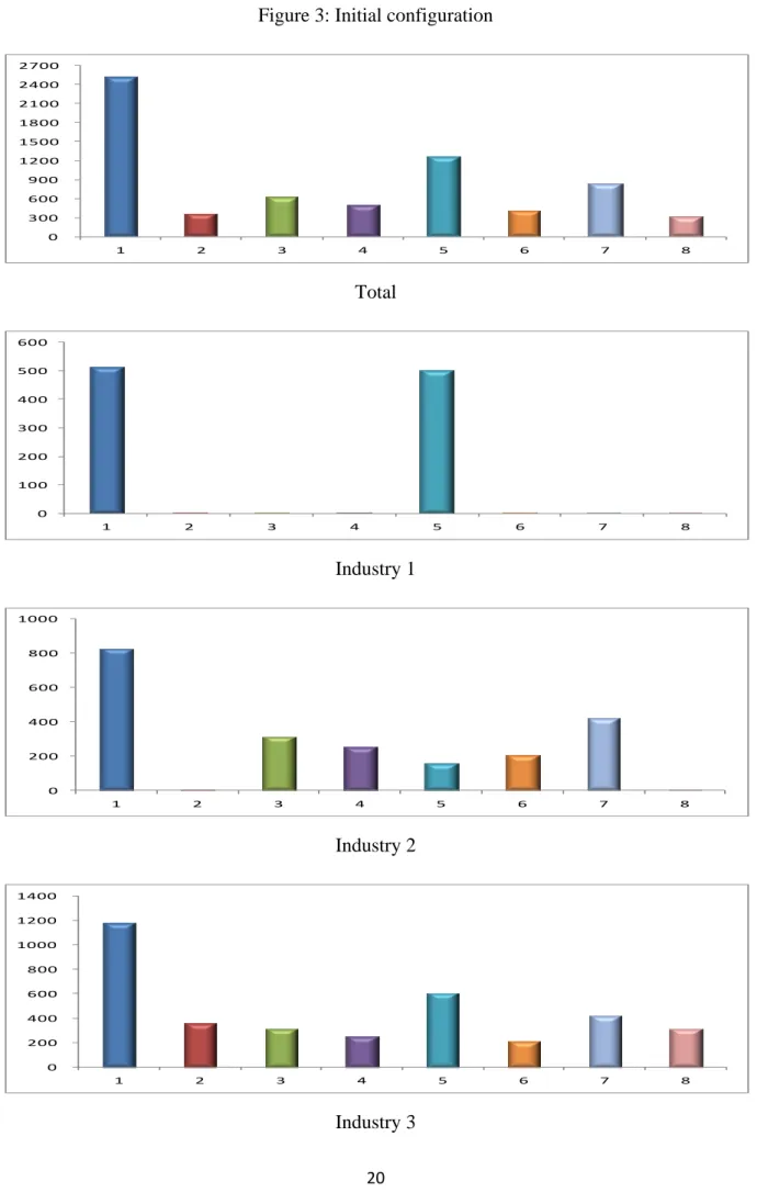
1 2,520 515 825 1,180 304 2 357 1 1 355 133 3 629 1 315 313 111 4 503 1 251 251 91 5 1,260 501 155 604 195 6 419 1 208 210 78 7 839 1 421 417 138 8 313 1 1 311 117
Figure 3 shows the initial configuration which satisfies both rank-size rule and central place theory. Figure 4 shows the results with higher transport costs in order to verify that the model is correctly set up. Figure 5 displays the situation after 200 rounds of iteration. Oddly, they do not seem to converge to symmetry. To remove any first nature advantage, land areas are reallocated among the cities. The land areas could be regarded as an inherent advantage a region possesses like climate features and raw material, as opposed to second nature which are the result of human actions to improve upon the first nature. Figure 6 demonstrates that the space economy now fast approaches symmetry. Figure 7 shows the state at round 200, with the cities almost equalized in all aspects.
We are now ready to study the population shrinkage. The rate of change is not city-specific; rather it is deemed to depend on the current size of the city in question. We consider two rather extreme cases. Figure 8 traces the changes when smaller cities shrink faster (Case A). In each period, natural changes occur according to the schedule for different city sizes and then followed by social changes caused by workers roaming across cities as specified in the model. Two opposing forces come into play. A city with larger centripetal force would gain population and vice versa. A general shrinking trend is apparent, but medium-order industry starts spilling onto two smallest cities previously overshadowed by the primate city. Figure 9 highlights the growing shares of the two smallest cities, while Figure 10 depicts the situation at round 10. How realistic is this prediction? The following excerpt provides a clue:
In the decade from 2000 to 2010 Detroit lost an astonishing 25% of its population… There are now about 60,000 empty houses… Detroit is now incredibly cheap, and that has drawn some rather pioneering types back into town [including] the largest internet mortgage company in America… You can buy a vast Victorian town-house in a perfectly pleasant area for $100,000 or a loft in somewhere a bit edgier for considerably less.4
Now suppose population shrinks with the larger cities dwindling faster (Case B). As Figure 11 illustrates, the process becomes very slow as the cities become small. Figures 12 and 13 show the city shares and their state at round 10, respectively. Nonetheless, a similar phenomenon occurs with the medium-order industry spreading to cities 2 and 8. In this model, hierarchy is partly disrupted as population shrinks.
Then, a couple of welfare analyses are performed. Figure 14 compares the utility levels under three different uniform rates of natural change. Initially, lower demand for land causes rent to go down boosting the utility. However, illusion is short lived because the markets start shrinking and suppressing wages. It is also better to maintain a low pace of population decline
4
17
in the long-term perspective. Finally, Figure 15 presents utility with varying rates. We compare two cases against the fixed rate of -5%. Case B clearly outperforms in the long run, implying the importance of sustaining the livability of smaller cities.
6. Conclusions
Since the early 1970s, balanced growth has been at the heart of Korea’s regional development policy. There has been, and will be, much discussion on the very necessity and proper forms of so-called balanced regional growth in Korea. In the face of the unprecedented event of an impending depopulation, a whole new approach and shift of paradigm are desperately needed. In this study, we can extract a number of interesting possibilities which enable us to better comprehend what would happen to the existing cities when the country’s population starts to shrink, while deriving useful policy implications for preserving the utility of residents.
People struggle against the “tyranny of distance”. In this paper, I raise the question of whether population shrinkage leads to changes in urban hierarchy in terms of their relative sizes and functions from the standpoint of the new economic geography. We have found some salient patterns in which small cities in the agglomeration shadow become relatively bigger as medium industries spill over on them. This result is quite robust against variation in the rates of natural change among cities.
There are many directions this study can be improved upon. Crozet (2004) focused on the forward linkage of individual location choices. The high barriers to migration hinder rapid evolution toward a core-periphery pattern, although this is less of an issue within a country. He considers migration costs and employment opportunities with a stochastic component within the framework of the EU. Although migrants follow market potentials for firms, the centripetal forces are quite limited due to high mobility costs. Consideration of employment probability and migration cost would certainly add a more realistic flavor to the present model.
Another meaningful direction to pursue is the agent-based microsimulation modeling. Fowler (2007) contrasted geographers’ criticism on the economists’ assumptions, determinism and dependence on analytic models against economists criticizing geographical economists for depending on simulation rather than analytical solutions, simplistic representation on the interaction between firms and lack of strong empirical evidence. He then postulates a situation where each firm and worker acts individually reflecting heterogeneous behavior. Most NEG models, including the present one, derive the number of firms in a given region from the size of the local labor market. It does not always have to be the case. Outside the equilibrium, firms and workers know the outcome of their decisions up to a point, but conditions would change as other firms and workers make their own decisions. After each move, if the sum of profits and losses is positive, an additional firm is spawned, while if it is negative, a firm will be removed. In other words, firms have bounded rationality, and are rewarded or dropped depending on their choice.
Including intermediate goods, while closer to reality, is much more involving, and it would be extremely difficult to find a set of parameter values that enables the equilibrium to satisfy both the rank-size rule and central place hierarchy. Nonetheless, Venables (1996) showed that a cumulative causation by final sector firms and intermediate goods suppliers can lead to a core-periphery structure even without labor mobility. The firms selling poorly differentiated goods remain dispersed while firms supplying highly differentiated products leave large cities and set up in the urban shadows.
With our model, one can also simulate and assess the impact of large-scale natural disasters that destroy cities and transportation networks. It can also be used to devise an optimal order of reconstruction that is crucial in recovering the pre-disaster level of city order and hierarchy. Lastly, we need to consider changing age structures in cities. Total fertility rates
18
in many regions are below the natural replacement level. Rising life expectancy means a higher share of the elderly population. Countries will have to reduce either the benefits of public pension or the coverage thereof. Decline of tax revenue and increases in the fiscal deficit mean negative shocks on productivity and a slowdown of economic growth. Conflicts among generations are thus inevitable.
19
Figure 1: Total fertility by major regions
Source: World Population Prospects, United Nations (2010)
Figure 2: Populations of Japan and Korea
Japan Korea Source: World Population Prospects, United Nations (2010)
20
Figure 3: Initial configuration
Total Industry 1 Industry 2 Industry 3 0 300 600 900 1200 1500 1800 2100 2400 2700 1 2 3 4 5 6 7 8 0 100 200 300 400 500 600 1 2 3 4 5 6 7 8 0 200 400 600 800 1000 1 2 3 4 5 6 7 8 0 200 400 600 800 1000 1200 1400 1 2 3 4 5 6 7 8
21
Figure 4: High transport costs with given land (up to 100 rounds)
Total Industry 1 Industry 2 Industry 3 0 1000 2000 3000 4000 5000 6000 7000 8000 1 4 7 10 13 16 19 22 25 28 31 34 37 40 43 46 49 52 55 58 61 64 67 70 73 76 79 82 85 88 91 94 97 100 8 7 6 5 4 3 2 0 200 400 600 800 1000 1200 1400 1 4 7 10 13 16 19 22 25 28 31 34 37 40 43 46 49 52 55 58 61 64 67 70 73 76 79 82 85 88 91 94 97 100 8 7 6 5 4 3 2 0 500 1000 1500 2000 2500 1 4 7 12 13 16 19 22 25 28 31 34 37 40 43 46 49 52 55 58 61 64 67 70 73 76 79 82 85 88 91 94 97 100 8 7 6 5 4 3 2 0 500 1000 1500 2000 2500 3000 3500 4000 1 4 7 10 13 16 19 22 25 28 31 34 37 40 43 46 49 52 55 58 61 64 67 70 73 76 79 82 85 88 91 94 97 10 0 8 7 6 5 4 3 2
22
Figure 5: High transport costs with given land (at round 200)
Total Industry 1 Industry 2 Industry 3 0 300 600 900 1200 1500 1800 2100 2400 2700 1 2 3 4 5 6 7 8 0 100 200 300 400 500 600 1 2 3 4 5 6 7 8 0 200 400 600 800 1000 1 2 3 4 5 6 7 8 0 200 400 600 800 1000 1200 1400 1 2 3 4 5 6 7 8
23
Figure 6: High transport costs with equal land (up to 100 rounds)
Total Industry 1 Industry 2 Industry 3 0 1000 2000 3000 4000 5000 6000 7000 8000 1 4 7 10 13 16 19 22 25 28 31 34 37 40 43 46 49 52 55 58 61 64 67 70 73 76 79 82 85 88 91 94 97 100 8 7 6 5 4 3 2 0 200 400 600 800 1000 1200 1 4 7 10 13 16 19 22 25 28 31 34 37 40 43 46 49 52 55 58 61 64 67 70 73 76 79 82 85 88 91 94 97 100 8 7 6 5 4 3 0 500 1000 1500 2000 2500 3000 1 4 7 12 13 16 19 22 25 28 31 34 37 40 43 46 49 52 55 58 61 64 67 70 73 76 79 82 85 88 91 94 97 10 0 8 7 6 5 4 3 0 1000 2000 3000 4000 1 4 7 10 13 16 19 22 25 28 31 34 37 40 43 46 49 52 55 58 61 64 67 70 73 76 79 82 85 88 91 94 97 100 8 7 6 5 4 3
24
Figure 7: High transport costs with equal land (at round 200)
Total Industry 1 Industry 2 Industry 3 0 300 600 900 1200 1500 1800 2100 2400 2700 1 2 3 4 5 6 7 8 0 100 200 300 400 500 600 1 2 3 4 5 6 7 8 0 200 400 600 800 1000 1 2 3 4 5 6 7 8 0 200 400 600 800 1000 1200 1400 1 2 3 4 5 6 7 8
25
Figure 8: Population shrinkage when small cities shrink faster (up to 30 rounds)
Total Industry 1 Industry 2 Industry 3 0 1000 2000 3000 4000 5000 6000 7000 8000 1 2 3 4 5 6 7 8 9 10 11 12 13 14 15 16 17 18 19 20 21 22 23 24 25 26 27 28 29 30 8 7 6 5 4 3 2 1 0 200 400 600 800 1000 1200 1 2 3 4 5 6 7 8 9 10 11 12 13 14 15 16 17 18 19 20 21 22 23 24 25 26 27 28 29 30 8 7 6 5 4 3 2 1 0 500 1000 1500 2000 2500 1 2 3 4 5 6 7 8 9 10 11 12 13 14 15 16 17 18 19 20 21 22 23 24 25 26 27 28 29 30 8 7 6 5 4 3 2 1 0 500 1000 1500 2000 2500 3000 3500 4000 1 2 3 4 5 6 7 8 9 10 11 12 13 14 15 16 17 18 19 20 21 22 23 24 25 26 27 28 29 30 8 7 6 5 4 3 2 1
26
Figure 9: Population shrinkage when small cities shrink faster (city shares)
Total Industry 1 Industry 2 Industry 3 0% 10% 20% 30% 40% 50% 60% 70% 80% 90% 100% 1 2 3 4 5 6 7 8 9 10 11 12 13 14 15 16 17 18 19 20 21 22 23 24 25 26 27 28 29 30 8 7 6 5 4 3 2 1 0% 10% 20% 30% 40% 50% 60% 70% 80% 90% 100% 1 2 3 4 5 6 7 8 9 10 11 12 13 14 15 16 17 18 19 20 21 22 23 24 25 26 27 28 29 30 8 7 6 5 4 3 2 1 0% 10% 20% 30% 40% 50% 60% 70% 80% 90% 100% 1 2 3 4 5 6 7 8 9 10 11 12 13 14 15 16 17 18 19 20 21 22 23 24 25 26 27 28 29 30 8 7 6 5 4 3 2 1 0% 10% 20% 30% 40% 50% 60% 70% 80% 90% 100% 1 2 3 4 5 6 7 8 9 10 11 12 13 14 15 16 17 18 19 20 21 22 23 24 25 26 27 28 29 30 8 7 6 5 4 3 2 1
27
Figure 10: Population shrinkage when small cities shrink faster (at round 10)
Total Industry 1 Industry 2 Industry 3 0 300 600 900 1200 1500 1800 2100 2400 2700 1 2 3 4 5 6 7 8 0 100 200 300 400 500 600 1 2 3 4 5 6 7 8 0 200 400 600 800 1000 1 2 3 4 5 6 7 8 0 200 400 600 800 1000 1200 1400 1 2 3 4 5 6 7 8
28
Figure 11: Population shrinkage when large cities shrink faster (up to 30 rounds)
Total Industry 1 Industry 2 Industry 3 0 1000 2000 3000 4000 5000 6000 7000 8000 1 2 3 4 5 6 7 8 9 10 11 12 13 14 15 16 17 18 19 20 21 22 23 24 25 26 27 28 29 30 8 7 6 5 4 3 2 1 0 200 400 600 800 1000 1200 1 2 3 4 5 6 7 8 9 10 11 12 13 14 15 16 17 18 19 20 21 22 23 24 25 26 27 28 29 30 8 7 6 5 4 3 2 1 0 500 1000 1500 2000 2500 1 2 3 4 5 6 7 8 9 10 11 12 13 14 15 16 17 18 19 20 21 22 23 24 25 26 27 28 29 30 8 7 6 5 4 3 2 1 0 500 1000 1500 2000 2500 3000 3500 4000 1 2 3 4 5 6 7 8 9 10 11 12 13 14 15 16 17 18 19 20 21 22 23 24 25 26 27 28 29 30 8 7 6 5 4 3 2 1
29
Figure 12: Population shrinkage when large cities shrink faster (city shares)
Total Industry 1 Industry 2 Industry 3 0% 10% 20% 30% 40% 50% 60% 70% 80% 90% 100% 1 2 3 4 5 6 7 8 9 10 11 12 13 14 15 16 17 18 19 20 21 22 23 24 25 26 27 28 29 30 8 7 6 5 4 3 2 1 0% 10% 20% 30% 40% 50% 60% 70% 80% 90% 100% 1 2 3 4 5 6 7 8 9 10 11 12 13 14 15 16 17 18 19 20 21 22 23 24 25 26 27 28 29 30 8 7 6 5 4 3 2 1 0% 10% 20% 30% 40% 50% 60% 70% 80% 90% 100% 1 2 3 4 5 6 7 8 9 10 11 12 13 14 15 16 17 18 19 20 21 22 23 24 25 26 27 28 29 30 8 7 6 5 4 3 2 1 0% 10% 20% 30% 40% 50% 60% 70% 80% 90% 100% 1 2 3 4 5 6 7 8 9 10 11 12 13 14 15 16 17 18 19 20 21 22 23 24 25 26 27 28 29 30 8 7 6 5 4 3 2 1
30
Figure 13: Population shrinkage when large cities shrink faster (round 10)
Total Industry 1 Industry 2 Industry 3 0 300 600 900 1200 1500 1800 2100 2400 2700 1 2 3 4 5 6 7 8 0 100 200 300 400 500 600 1 2 3 4 5 6 7 8 0 200 400 600 800 1000 1 2 3 4 5 6 7 8 0 200 400 600 800 1000 1200 1400 1 2 3 4 5 6 7 8
31
Figure 14: Utility with uniform rates
Figure 15: Utility with varying rates 12 14 16 18 20 22 24 1 2 3 4 5 6 7 8 9 10 11 12 13 14 15 16 17 18 19 20 21 22 23 24 25 26 27 28 29 30 - 1% - 10% - 5% 14 15 16 17 18 19 20 21 22 1 2 3 4 5 6 7 8 9 10 11 12 13 14 15 16 17 18 19 20 21 22 23 24 25 26 27 28 29 30 Case B Fixed Case A