Market power of China's state-owned firms :
evidence from manufacturing firm-level data
著者
Hashiguchi Yoshihiro
権利
Copyrights 2020 by author(s)
journal or
publication title
IDE Discussion Paper
volume
779
year
2020-03
INSTITUTE OF DEVELOPING ECONOMIES
IDE Discussion Papers are preliminary materials circulated to stimulate discussions and critical comments
Keywords: Markups, China’s state-owned firms, Manufacturing firm-level data JEL classification: D22, D24, L11, P21
* Research Fellow, Economic Modelling Studies Group, Development Studies Center, IDE ([email protected])
IDE DISCUSSION PAPER No. 779
Market power of China's
State-owned Firms: Evidence from
Manufacturing Firm-level Data
Yoshihiro HASHIGUCHI*
March 2020
Abstract
There has been a great discussion about a phenomenon: Guojin Mintui (i.e., the state advances, the private sector retreats) since the latter half of the 2000s. Has the state-owned sector been expanding and undermining private enterprises? To address this issue, this paper estimates changes in markups of China's state-owned firms from 2003 to 2007, using manufacturing firm-level data. It is found that the relative markup of the state sector is smaller than those of the private and foreign sectors, while it tends to steadily increase and be catching up with the private and foreign sector during 2004--2007; However, the catching up process is not observed in surviving firms. This implies that the exit of the state-owned firms with lower markups causes the increase in the average markups of the state sector. In terms of the relative markups in the manufacturing sector for 2003 to 2007, this study does not support the argument of Guojin Mintui.
The Institute of Developing Economies (IDE) is a semigovernmental, nonpartisan, nonprofit research institute, founded in 1958. The Institute merged with the Japan External Trade Organization (JETRO) on July 1, 1998. The Institute conducts basic and comprehensive studies on economic and related affairs in all developing countries and regions, including Asia, the Middle East, Africa, Latin America, Oceania, and Eastern Europe.
The views expressed in this publication are those of the author(s). Publication does not imply endorsement by the Institute of Developing Economies of any of the views expressed within.
INSTITUTE OF DEVELOPING ECONOMIES (IDE), JETRO
3-2-2, WAKABA,MIHAMA-KU,CHIBA-SHI
CHIBA 261-8545, JAPAN
©2020 by author(s)
No part of this publication may be reproduced without the prior permission of the author(s).
Market power of China’s state-owned firms
—Evidence from manufacturing firm-level data—
Yoshihiro Hashiguchi
∗March 2020
Abstract
There has been a great discussion about a phenomenon: Guojin Mintui (i.e., the state advances, the private sector retreats) since the latter half of the 2000s. Has the state-owned sector been expanding and undermining private enterprises? To address this issue, this paper estimates changes in markups of China’s state-owned firms from 2003 to 2007, using manufacturing firm-level data. It is found that the relative markup of the state sector is smaller than those of the private and foreign sectors, while it tends to steadily increase and be catching up with the private and foreign sector during 2004–2007; However, the catching up process is not observed in surviving firms. This implies that the exit of the state-owned firms with lower markups causes the increase in the average markups of the state sector. In terms of the relative markups in the manufacturing sector for 2003 to 2007, this study does not support the argument of Guojin Mintui.
Keywords: Markups, China’s state-owned firms, Manufacturing firm-level data JEL classification: D22, D24, L11, P21
1
Introduction
Since China’s reform and open-door policies in 1978, various policy measures have been taken to reform the inefficient production systems of the state-owned enterprises (SOEs). In the begin-ning, the SOEs had been traditionally considered as the foundation of Socialist economy, and drastic reform of the SOEs were not implemented. Despite the reform, SOEs’ profit rate had continued to decline in the 1980s. Furthermore, inflation and the Tiananmen Square incident caused a serious blow to Chinese economy. China had been forced to review their strategy for economic growth. After Deng Xiaoping’s southern tour of China in 1992, a liberalization pol-icy for economic development was given priority over the preservation of traditional Socialist economy in order to get over the deep recession. The adoption of the liberalization policy led to a massive entry of private sector firms in a wide range of fields and consequently the SOEs sector had contracted their presence in Chinese economy in the 1990s.
The shrinkage of the state-owned sector and expansion of the private sector in the 1990s is usually described in Chinese as Guotui Minjin (i.e., the private advances, the state sector retreats). In a sense, this phenomenon comes as no surprise because China’s government has advanced the reform based on market principles. However, in recent years, many scholars have reported a phenomenon running counter to Guotui Minjin, that is, Guojin Mintui (i.e., the state advances, the private sector retreats).1) For example, it is reported that SOEs colluded with government are likely to use public authority to beat private competitors and that SOEs have advantageous access to factor resources such as capital from bank loans, subsidies, and land (Kato, 2012; Watanabe, 2013). Such cases indicate a possibility that there exist unfair competitive conditions between the state and non-state sector firms and that enables SOEs to have larger market power than the private sector.
Has the state-owned sector been expanding in recent years? From a qualitative perspective, the presence of SOEs seems to be increasing after 2003, because after Hu Jintao was elected as the president of China in 2002, the State Asset Supervision and Administration Commis-sion (SASAC) was created in 2003, and SASAC began to increase in the size and importance of the SOEs (Naughton, 2011). As is symbolized by the establishment of SASAC, China’s government had revealed a policy to firmly maintain the important presence of the SOEs since then. Furthermore, it is said that many social and economic policies for regional and indus-trial development, conducted in the 2000s, largely contributed to increasing the presence of SOEs (Naughton, 2011; Kato, 2012). However, the above argument lacks substantial statistical evidence. As Kato (2012) and Marukawa (2015) pointed out, judging from the official macroe-conomic data from 1998 to 2008, the share of SOEs tends to decrease in the number of firms, employees, value added, and total assets. By industrial sector, it dramatically decreased in the manufacturing, wholesale and retail industries. For the period from 2009 to 2011, SOEs was slightly increasing in their total number and asset share (Marukawa, 2015). And the share of SOEs was increasing in public and service sectors. In sum, according to previous studies, the expansion of SOEs is observed in the service sector after the 2009 global financial crisis, while that is not observed in the manufacturing sector at least before the crisis. The private sector has an overwhelmingly larger number of firms than the state sector and then, it does not seem to take place Guojin Mintui (the state advances, the private sector retreats).
However, as will be mentioned below, the firm size of SOEs is much greater than that of the private sector firms and it tends to increase over time. And there are several studies reporting that the state-owned sector is expanding and undermining private firms. How much influence do SOEs have in China’s economy where there exists both small number of large SOEs and large number of small private firms? This study attempt to revisit this issue from the viewpoint of market power. Market power is typically measured by markups (Hall, 1986; De Loecker and Warzynski, 2012). The author uses China’s manufacturing firm-level data from 2003 to 2007 to estimate firm-level markups and to compare them between the state-owned, domestic private, and foreign sectors. As a result, it is found that the relative markups of the state sector are smaller than those of the private and foreign sectors, while the markups of the state-owned sector tend to steadily increase and be catching up with the private and foreign firms during 2004–2007; However, the catching up process is not observed in surviving firms, implying that the exit of the state-owned firms with lower markups causes the increase in the average
markups of the state-owned sector. From the perspective of markups, it seems not to take place the expansion of SOEs in the manufacturing sector in the latter half of the 2000s.
The contribution of this paper is twofold. First, to the best of my knowledge, this study is the first to investigate the presence of SOEs in terms of the firm-level markups. Markups are typically used to represent the magnitude of market power which is the ability to control its product price in the market and is able to capture the presence and influential power of SOEs. As a result, the author finds new evidence that the markups of SOEs are significantly smaller than the private and foreign sectors during the period from 2004 to 2007, and the average markups in the SOEs tends to be increasing because of exiting SOEs with lower markups. Second, the author proposes a new nonparametric estimation strategy for the estimation of markups. While the famous methodology for markup estimation proposed by De Loecker and Warzynski (2012) requires us to estimate a firm-level production function, this paper’s nonparametric method enable us to estimate markups without identifying a production function. Because there is a fundamental difficulty in the estimation of production functions (Ackerberg, Caves, and Frazer, 2015; Gandhi, Navarro, and Rivers, 2020), this nonparametric approach is useful and works in the estimation of markups.
The remainder of this paper is organized as follows. Section 2 describes an empirical frame-work for the estimation of markups. Section 3 describes data used in the estimation, Section 4 reports the estimation results, and Section 5 concludes.
2
An Empirical Model to Estimate markups
This section shows an empirical framework to derive and estimate firm-level markups. Follow-ing the seminal paper by De Loecker and Warzynski (2012), the deviation is based on standard cost minimization conditions for a variable input free of adjustment costs. The derived markups are expressed by the cost share of a variable input and the output elasticity with respect to a variable input. After the author clarifies the representation of markups, an empirical strategy for the estimation of markups is discussed.
2.1
Deriving firm-level markups
Let us consider that a firm i at period t operates through discrete time t and produces an output using capital Kit, labor Lit, and intermediate inputs Mit. The relationship between these inputs
and output is expressed as
Qit= F(Kit, Lit, Mit) exp{ωit} (1)
whereωit is the anticipated productivity level which represents the types of technology,
infor-mation, knowledge or situations of the firm i that affect its productivity and can be observed by the firm at the beginning of each period, but not be observed by the econometrician. Qit
is an output anticipated by firm i at t. The actual and observed output Yit can be described by
including the effect of an unanticipated productivity shock εitwhich cannot be observed by firm
i before making its input decisions for period t:
Firm i’s cost minimization problem can be represented by the following Lagrangian func-tion:
L≡ ritKit+ witLit+ ρitMit+ λit[Qit− F(·) exp{ωit}] (3)
where rit, witandρitdenote unit prices of capital, labor, and intermediate inputs, respectively. It
is assumed that labor and capital are quasi-fixed inputs and predetermined at period t because adjustment costs exist in these inputs (e.g., hiring/firing, job training, or machine installation costs). On the other hand, intermediate input Mit is assumed to be flexible and there are no
adjustment costs in Mit. These assumptions imply that, at the beginning of each period, firm i
observesωitand chooses the level of Mit to minimize the firm’s cost, under the predetermined
levels of labor, capital, andωit. The first order condition of the cost minimization problem is
ρit− λit
∂F(·) exp{ωit}
∂Mit
= 0. (4)
Multiplying both side of Equation (4) by Mit/pitYityields the observed intermediate cost share
equation: Sit≡ ρitMit pitYit = λit pit ∂F(·) exp{ωit} ∂Mit Mit Yit = λit pit ∂F(·) exp{ωit} ∂Mit Mit F(·) exp{ωit+ εit} = λit pit ∂F(·) ∂Mit Mit F(·) 1 exp{εit} = µ1 it G(Kit, Lit, Mit) 1 exp{εit} G(·) ≡ ∂F(·) ∂Mit Mit F(·) µit≡ pit/λit (5)
where Sit is the cost share of the intermediate input Mit, pit is output price, and G(·) is the
elasticity of output with respect to Mit. Because the Lagrange multiplier λit is equal to the
marginal cost (MCit) under the first order condition,µitcan be rewritten as
µit = pit/MCit = ( 1− 1 νit )−1 (6) whereνit ≡ − pit Yit dYit
d pit is the price elasticity of demand, indicating firm i’s market power which
means the ability to control its product price in the market. If firm i faces a perfectly competitive market (i.e., νit = ∞), then µit ≡ pit/λit = 1. In other words, µit represents firm’s profitabilty.
Becauseµitis the ratio of a selling price and marginal production costs, firms selling a product
at a relatively high price compared to their marginal costs can be considered as profitable. If firm i has market power (νit < ∞), then µit is greater than 1. In general, the smallerνit is, the
larger the degree of market power (µit).
This study estimatesµit at firm-level and examines whether the market power of the
2.2
Estimation of Markups
To estimate markupsµit, De Loecker and Warzynski (2012) proposed using an estimate of the
output elasticity of a variable input free of adjustment costs, such as
ˆ µit = ˆ Git Sitexp{ˆεit} (7)
where ˆGit is an estimated output elasticity of a variable input, and ˆεit is a residual which can
be recovered from the estimated production function. Their approach requires us to estimate the output production function including both quasi fixed inputs with adjustment costs (e.g., labor and capital inputs) and variable inputs free of adjustment costs (e.g., intermediate inputs). However, there is a fundamental difficulty in the estimation of output production functions, referred to as the simultaneity problem (Ackerberg, Caves, and Frazer, 2015; Gandhi, Navarro, and Rivers, 2020).
In this paper, the author proposes an alternative nonparametric approach which does not require us to estimate production function to obtain markups estimates.2)Taking the logarithm for both side of Equation (5) yields
ln Sit= − ln µit+ ln G(Kit, Lit, Mit)− εit
= −˜µit+ g(kit, lit, mit)+ ηit
(8)
where ˜µit ≡ ln µit, g(kit, lit, mit) ≡ ln G(Kit, Lit, Mit), and ηit ≡ −εit. The lower case letters of
inputs denote the logarithm of inputs. A polynomial expression is used to approximate the log elasticity g(kit, lit, mit), and the polynomial expression can be divided into a constant and varying
components:
g(kit, lit, mit)≈ poly(kit, lit, mit)
= c + polyv(k
it, lit, mit)
(9)
where poly(kit, lit, mit) represents a polynomial series of kit, lit, and mit; and c and polyv(kit, lit, mit)
are the constant and varying components for i and t.3)To investigate the differences of the market power ˜µitbetween the ownership sectors, ˜µitis replaced as follows:
˜
µit = α0+ αpPrivateit+ αfForeignit+ βexExpdmit+ S′itγ + T′itθ + eit (10)
whereα0 and eitdenote a constant term and an unanticipated price shock which cannot be
ob-served by firm i before making its input decisions for period t. The terms Privateitand Foreignit
denote the dummy variables of the ownership sectors. Firms are divided by three ownership groups: State, Private+, and Foreign, where State denotes the set of SOEs, including state-owned enterprises and solely state-funded corporations; Private+ denotes the set of domestic and non-state-owned firms, including collective-owned firms (and other hybrids) and privately
2)This approach is inspired by Gandhi, Navarro, and Rivers (2020) who propose a nonparametric identification
strategy for the estimation of output production functions.
3)The application of a polynomial series for the elasticity function follows the nonparametric identification
funded enterprises; and Foreign denotes the set of firms with funds from Hong Kong, Macao, and Taiwan and those that are purely foreign-funded enterprises. The ownership dummies are defined as Privateit = 1 if firm i ∈ Private+ and Foreignit = 1 if firm i ∈ Foreign. The forth term
ExpDmi denotes a exporting firm dummy which is eqaul to 1 if firm i’s exports are observed at any point during the observation periods (2003–2007). The vector of Sit denotes the set of
the firm size quintile dummies. Firms are divided by five groups identifying the quintile of firm output at period t. Specifically, the vector Sitis defined as
Sit=
[
Sizedm2it Sizedm3it Sizedm4it Sizedm5it
]′ ,
where Sizedm2it–Sizedm5itindicate the firm size dummies from second to fifth quintile ranges.4)
The vector Tit is the set of time dummies. Finally, eit is assumed to be orthogonal to these
dummy variables in Equation (10).
Substituting Equations (9) and (10) into (8) and including industrial and regional fixed ef-fects, the following estimation equation is obtained:
ln Sit= ¯c − αpPrivateit− αfForeignit− βexExpdmit− S′itγ − T′itθ
+ polyv(k
it, lit, mit)+ IndustryDm + ProvinceDm + ¯ηit,
(11)
where ¯c ≡ c − α0, ¯ηit ≡ ηit− eit, IndustryDm and ProviceDm denote the set of 3-digit
indus-trial dummies and the province level regional dummies, respectively. This is the benchmark estimation model in this study. The term ¯ηit is treated as an error term. As mentioned above,
¯
ηit is the unanticipated shocks for firm i and not correlated with these dummy variables and
polyv(kit, lit, mit) in the estimation equation. Although we cannot identify the absolute level of
the market power for each ownership sector becauseα0cannot be identified, Equation (11) en-ables us to estimate the relative market power of the private and foreign sectors compared to the state-owned sector without estimating gross output production functions.
In addition, to investigate changes in the relative market power for each ownership sector, the interaction terms between the ownership and time dummies are introduced:
ln Sit = ¯c − Privateit× T′itαp− Foreignit× Tit′αf − βexExpdmit− S′itγ − T′itθ
+ polyv
(kit, lit, mit)+ IndustryDm + ProvinceDm + ¯ηit,
(12)
whereαpandαf represent vectors of parameters indicating changes in the relative market power
for the Private+ and Foreign sectors, respectively.
In this study, the author estimates Equations (11) and (12) using China’s manufacturing firm-level data, and examines whether the market powers of the Private+ and Foreign sector firms is greater than that of the State sector firms, and how the relative market powers change over time.
3
Data Description
Data used for the estimation is China’s manufacturing firm-level panel data from 2003 to 2007, drawn from the annual survey of industrial enterprises conducted by the National Bureau of
Statistics. The survey covers all industrial firms with sales of over 5 million RMB. The data set consists of three industries: mining, manufacturing, and public utilities. This study uses the manufacturing industry data. The data contains information on a series of firms’ IDs. However, the IDs are often missing or changes over time. In this study, following Hashiguchi (2020), the author creates a new series of firms’ ID for constructing the panel data by using the attributes of firms.5)
The variables in the estimation equation (11) are constructed as follwos: Sit is the share
of the total intermediate inputs in the total gross output, Kit is the total fixed assets, Lit is the
number of employees, and Mit is the total intermediate inputs. The deflator for Mit are based
on the input deflators provided by Brandt, et al. (2012).6) The deflator for total fixed assets is constructed using the province-level investment deflator which is obtained the China Statistical Yearbook.
The following firms are removed as outliers from the database: 1) firms with a non-positive value for gross outputs, total fixed assets, employees, or total intermediate input; 2) firms whose gross output per worker or fixed assets per worker in t is more than 1000 times or less than 0.001 the value in t− 1; or 3) firms in Tobacco and nuclear-related industries. In addition, firms with
Sit > 1 are also removed from the database.
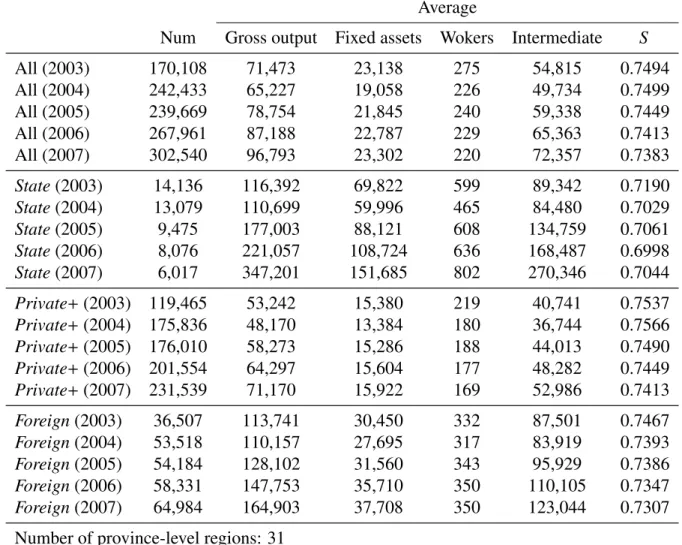
[– Table 1 –]
Table 1 shows the summary statistics. The number of state-owned firms is much lower than those of domestic private and foreign sector firms and a sharp decrease in numbers by 58% from 2003 to 2007, while the numbers of domestic private and foreign firms have increased over five years. The Private+ sector has the highest number of firms and accounted for 76% of the total in 2007. However, its gross output per firm is nearly five times lower than that of state-owned firms in 2007, indicating that most of the domestic private firms are very small in operating capacity compared to state-owned and foreign firms. The firm size of SOEs, measuring gross output per firm, is much greater than that of the private sector firms and it tends to increase over time. There exists both small number of large state-owned firms and large number of small domestic private firms in China’s manufacturing sector.
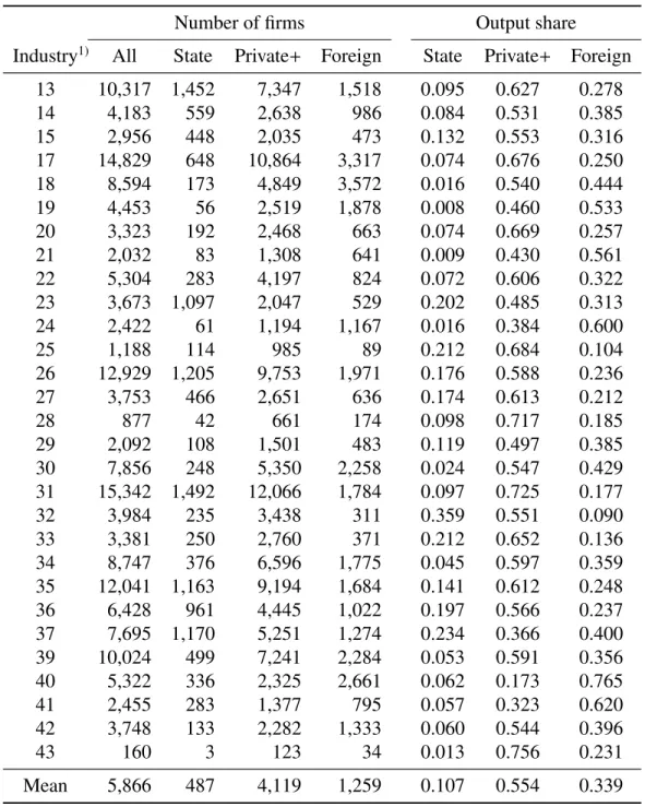
[– Table 2 –]
[– Table 3 –]
Tables 2 and 3 report the number of firms and the market share by 2-digit industrial sector for 2003 and 2007. China’s 2-digit industrial classification is described in Appendix Table 1. Market shares are measured by firm-level gross output values. Average market shares for the
State, Private+ and Foreign sectors are 10.6%, 55.5%, and 33.9% in 2003, and 5.6%, 59.1%,
and 35.3% in 2007, respectively. While the average firm size of the State sector firms is much higher than the Private+ and Foreign sector firms, the market shares of the State sector are the
5)For more details about the construction of the panel data, refer to Hashiguchi (2020). 6)See their online appendix: http://www.econ.kuleuven.be/public/n07057/china/.
smallest in most of industries and tend to decrease from 2003 to 2007.
Appendix Tables 2 and 3 show the market share of top five largest firms and the Herfindahl-Hirschman Index (HHI), respectively. Market concentration has been slightly decreasing in the manufacturing sector. Higher concentration is found in industries of oil processing, coking, and nuclear manufacturing (#25), chemical fiber manufacturing (#28), rubber product (#29), and removal and processing of obsolete resource and material (#43). Textile industry (#17) has smaller market concentration, while it shows the highest increase in the market concentration during 2003–2007. Overall, the market concentration tends to slightly decrease in many 2-digit industrial sectors, implying that the market competitiveness has been increasing in the manufacturing sector.
4
Estimation Results
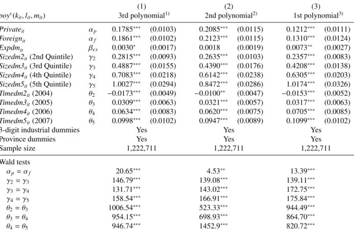
[– Table 4 –]
Table 4 shows the estimation result of Equation (11). The polynomial function polyv(kit, lit, mit)
is defined by using first, second, and third order polynomial series. The third order polynomial, which is the most flexible among them, is employed as the benchmark model in this study. It is noted that the estimation results are robust with respect to the order of polynomial expression.
The coefficients of Privateit and Foreignitsectors are 0.178 and 0.186, respectively, both of
which are statistically significant at 99%. This indicates that the markupµit of the State sector
is, on average throughout the period 2003–2007, relatively smaller than those of Privateit and
Foreignit sectors. The coefficient of the export dummy (Expdmit) is slightly positive (0.003) and significant at 90%. China’s exporting firms do not necessarily have a large market power compared to non-exporting firms, which is the opposite results of De Loecker and Warzynski (2012). Estimates of the firm size dummies (Sizedm2it–Sizedm5it) are 0.282, 0.489, 0.708,
and 1.003, respectively, and the Wald tests for the equality of estimated parameters show a statistically significant difference between those estimates. This indicates that larger firms tend to have larger markups. The economies of scale may affect the estimate of markups. Estimates of time dummies (Timedm2it–Timedm5it) tend to increase over time. Although the estimate of
Timedm2itis negative indicating that the markup decreases from 2003 to 2004, as the result of
the Wald tests shows, the markup significantly increases on average during 2004–2007.
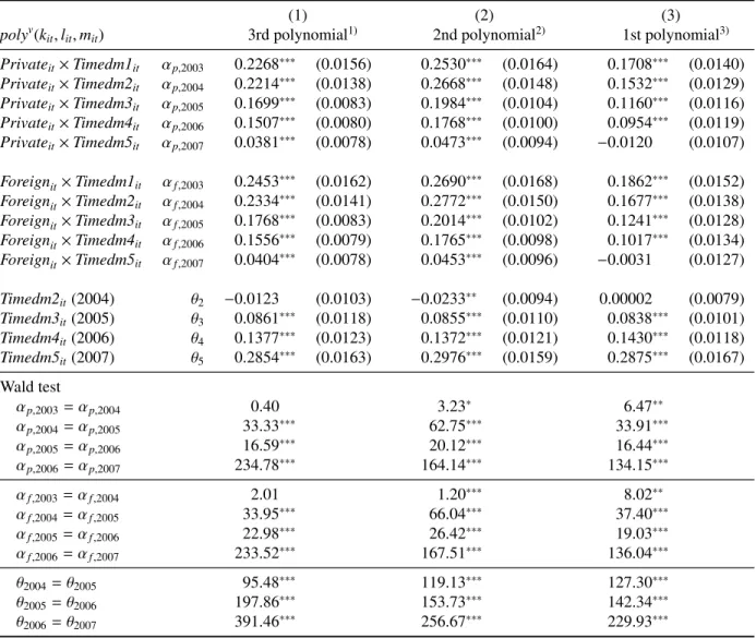
[– Table 5 –]
[– Figure 1 –]
Table 5 shows the estimation result of Equation (12) which includes the interaction terms between the ownership and time dummies. This table reports only the estimates of time dum-mies and their interaction terms to focus on changes in the relative markups for each ownership sector. The relative markups power of the private and foreign sectors tend to decrease over time, while those of the state-owned sector increases after 2004. As shown in the results of the Wald
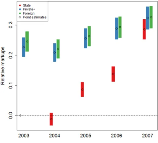
tests, while changes in the market power from 2003 to 2004 are not statistically significant, the markups tend to significantly increase in the state sector and to decrease in the private and foreign sectors after 2004. Figure 1 demonstrates a time series plots of the estimated relative markups, which are normalized at zero in the State sector in 2003.7) It is found that, although the relative markups of the state sector are still smaller in 2007 than those of the private and foreign sectors, the market power of the State sector has been steadily increasing and catching up with the private and foreign sectors since 2004.
[– Table 6 –]
[– Figure 2 –]
To investigate whether this catching up process is driven by surviving firms during the pe-riod for 2003–2007, the author constructs a dummy variable which is equal to one if a firm is observed in both 2003 and 2007, and estimates markups for surviving firms by ownership sec-tor. Table 6 report the estimation results and Figure 2 plots changes in the relative markups of surviving firms. While the markups of surviving SOEs is still smaller than those of the private and foreign sectors, the catching up process shown in Figure 1 almost disappears in Figure 2. This implies that a large increase of markups in the State sector is likely to be driven by the exit of SOEs with lower markups.
In the benchmark model, the collectively owned firms are included in the private sector. However, in general, those firms belong to a group of publicly owned firms, and their market power may differ from the privately funded firms. Then, the author divides the private sec-tor firms into the collectively owned and privately funded firms, and examines whether this modification affects the results of the benchmark model. Appendix Tables 5 and 6 report the estimation results. It is found that the relative markup of collectively owned firms is close to the same as those of privately funded firms, suggesting that the benchmark result is robust to this modification.
5
Concluding remarks
Over the past few years, many researchers have shown an interest in the phenomenon: Guojin
Mintui (i.e., the state advances, the private sector retreats). The official macroeconomic data
from 1998 to 2008 shows the share of SOEs tends to decrease in the number of firms, employees, value added, and total assets (Kato, 2012; Marukawa, 2015). By industrial sector, it dramatically decreased in the manufacturing, wholesale and retail industries. It seems that the presence of SOEs was not increasing but rather decreasing in the 2000s. However, no studies have been done to examine the market power of SOEs. This paper revisits the Guojin Mintui issue by estimating the market power, measured by markups, for the state-owned, domestic private,
7)The relative markups capture a distance from the reference constant term (¯c = c − α
0) which includesα0
indicating the absolute value of markups for the state-owned sector in 2003. Unfortunately, we cannot identifyα0
in the regression, implying that the absolute values of markups cannot be measured. To plot the relative markups, the constant term is conveniently normalized at zero by the author.
and foreign sector firms, using China’s manufacturing firm-level data from 2003 to 2007. To estimate the markups, the author proposed a new nonparametric approach in stead of the method of De Loecker and Warzynski (2012). While the author derives markups relying on standard cost minimization conditions for a variable input as is the case of De Loecker and Warzynski (2012), this paper’s approach does not need to estimate production functions to obtain markups. The author found that (1) the markups in the manufacturing sector on average were increas-ing durincreas-ing the period from 2004 to 2007, (2) the relative markups of SOEs are smaller than those of the private and foreign sector firms through the period, (3) the relative markups of SOEs tended to steadily increase and be catching up with the private and foreign sectors during 2004–2007, and (4) the catching up process is not observed in surviving firms, implying that the exit of the state-owned firms with lower markups causes the increase in the average markups of the state sector. In terms of the relative markups in the manufacturing sector for 2003 to 2007, this study does not support the argument of Guojin Mintui.
The persistent lower relative markup in the SOEs suggest possibilities that (1) the SOEs are simply less profitable than the private and foreign firms, (2) the inability of market selection to push less productive SOEs out of the market, and (3) SOEs engage in strategic dumping to obtain scale benefits and market shares (Caselli, Schiavo, and Nesta, 2018). Government subsidies to SOEs and/or a financial system advantageous to SOEs may hinter market selection and cause less profitable SOEs to survive in the market. Behind the lower markup in SOEs, there might be resource misallocation among the ownership sectors.
It is noted that the SOEs’ market power may have been more increasing since the global financial crisis in 2008. Chinese central government announced a 4 trillion RMB (US $586 billion) public investment in November 2008 to get out of the economic crisis. And the local government also expanded public works spending by taking advantage of the active economic stimulus policies of the central government. The series of the public investment policies can significantly increase the presence of Chinese government through the state-owned firms. While this study shows a trend of the SOE’s markups during the period from 2003 to 2007, this is quite likely to change after 2008. We need further research for the market structure and the operating environment of firms in China.
References
Ackerberg, D. A., K. Caves, andG. Frazer (2015): “Identification Properties of Recent
Pro-duction Function Estimators,” Econometrica, 83(6), 2411–2451.
Caselli, M., S. Schiavo,andL. Nesta (2018): “Markups and markdowns,” Economics Letters,
173, 104 – 107.
De Loecker, J.,andF. Warzynski (2012): “Markups and Firm-Level Export Status,” American Economic Review, 102(6), 2437–71.
Gandhi, A., S. Navarro,andD. A. Rivers (2020): “On the Identification of Gross Output
Pro-duction Functions,” Journal of Political Economy, forthcoming.
Hall, R. E. (1986): “Market Structure and Macroeconomic Fluctuations,” Brookings Papers on
Economic Activity, 1986(2), 285–338.
Kato, H. (2012): “The Present Stage of China’s Capitalism (in Japanese),” Journal of
Eco-nomics& Business Administration (The Kokumin-keizai zasshi), 206(2), 15–32.
Lardy, N. R. (2019): The state strikes back: The end of economic reform in China? Peterson Institute for International Economics.
Marukawa, T. (2015): “China Heading from the Social Capitalism to the Mixed-ownership Economy (in Japanese),” Japanese Journal of Comaparative Economics, 52(1), 47–57. Naughton, B. (2011): “China’s Economic Policy Today: The New State Activism,” Eurasian
Geography and Economics, 52, 313–329.
Watanabe, M. (2013): “Vigorous Entry and Cash Constraint: Entrepreneur’s Innovation Dodg-ing State Capitalism (in Japanese),” China 21, 38, 27–50.
Table 1: Summary statistics1) Average
Num Gross output Fixed assets Wokers Intermediate S
All (2003) 170,108 71,473 23,138 275 54,815 0.7494 All (2004) 242,433 65,227 19,058 226 49,734 0.7499 All (2005) 239,669 78,754 21,845 240 59,338 0.7449 All (2006) 267,961 87,188 22,787 229 65,363 0.7413 All (2007) 302,540 96,793 23,302 220 72,357 0.7383 State (2003) 14,136 116,392 69,822 599 89,342 0.7190 State (2004) 13,079 110,699 59,996 465 84,480 0.7029 State (2005) 9,475 177,003 88,121 608 134,759 0.7061 State (2006) 8,076 221,057 108,724 636 168,487 0.6998 State (2007) 6,017 347,201 151,685 802 270,346 0.7044 Private+ (2003) 119,465 53,242 15,380 219 40,741 0.7537 Private+ (2004) 175,836 48,170 13,384 180 36,744 0.7566 Private+ (2005) 176,010 58,273 15,286 188 44,013 0.7490 Private+ (2006) 201,554 64,297 15,604 177 48,282 0.7449 Private+ (2007) 231,539 71,170 15,922 169 52,986 0.7413 Foreign (2003) 36,507 113,741 30,450 332 87,501 0.7467 Foreign (2004) 53,518 110,157 27,695 317 83,919 0.7393 Foreign (2005) 54,184 128,102 31,560 343 95,929 0.7386 Foreign (2006) 58,331 147,753 35,710 350 110,105 0.7347 Foreign (2007) 64,984 164,903 37,708 350 123,044 0.7307 Number of province-level regions: 31
Number of 3-digit industrial sectors: 159
1)Outliers are excluded. S denote the share of total intermediate input in the total gross output. Num is the
num-ber of firms. State denotes the set of owned firms, including owned enterprises and solely state-funded corporations. Private+ denotes the set of domestic and non-state-owned firms, including collective-owned firms (and other hybrids) and privately funded enterprises. Foreign denotes the set of firms with funds from Hong Kong, Macao, and Taiwan and those that are purely foreign-funded enterprises.
Table 2: Number of firms and output share by industry in 2003
Number of firms Output share
Industry1) All State Private+ Foreign State Private+ Foreign
13 10,317 1,452 7,347 1,518 0.095 0.627 0.278 14 4,183 559 2,638 986 0.084 0.531 0.385 15 2,956 448 2,035 473 0.132 0.553 0.316 17 14,829 648 10,864 3,317 0.074 0.676 0.250 18 8,594 173 4,849 3,572 0.016 0.540 0.444 19 4,453 56 2,519 1,878 0.008 0.460 0.533 20 3,323 192 2,468 663 0.074 0.669 0.257 21 2,032 83 1,308 641 0.009 0.430 0.561 22 5,304 283 4,197 824 0.072 0.606 0.322 23 3,673 1,097 2,047 529 0.202 0.485 0.313 24 2,422 61 1,194 1,167 0.016 0.384 0.600 25 1,188 114 985 89 0.212 0.684 0.104 26 12,929 1,205 9,753 1,971 0.176 0.588 0.236 27 3,753 466 2,651 636 0.174 0.613 0.212 28 877 42 661 174 0.098 0.717 0.185 29 2,092 108 1,501 483 0.119 0.497 0.385 30 7,856 248 5,350 2,258 0.024 0.547 0.429 31 15,342 1,492 12,066 1,784 0.097 0.725 0.177 32 3,984 235 3,438 311 0.359 0.551 0.090 33 3,381 250 2,760 371 0.212 0.652 0.136 34 8,747 376 6,596 1,775 0.045 0.597 0.359 35 12,041 1,163 9,194 1,684 0.141 0.612 0.248 36 6,428 961 4,445 1,022 0.197 0.566 0.237 37 7,695 1,170 5,251 1,274 0.234 0.366 0.400 39 10,024 499 7,241 2,284 0.053 0.591 0.356 40 5,322 336 2,325 2,661 0.062 0.173 0.765 41 2,455 283 1,377 795 0.057 0.323 0.620 42 3,748 133 2,282 1,333 0.060 0.544 0.396 43 160 3 123 34 0.013 0.756 0.231 Mean 5,866 487 4,119 1,259 0.107 0.554 0.339
Table 3: Number of firms and output share by industry in 2007
Number of firms Output share
Industry1) All State Private+ Foreign State Private+ Foreign
13 17,509 475 14,597 2,437 0.021 0.695 0.284 14 6,360 146 4,808 1,406 0.030 0.580 0.390 15 4,254 159 3,408 687 0.064 0.570 0.366 17 27,279 221 21,536 5,522 0.019 0.741 0.241 18 14,421 91 8,385 5,945 0.010 0.536 0.454 19 7,331 17 4,614 2,700 0.003 0.493 0.504 20 7,676 78 6,561 1,037 0.012 0.793 0.194 21 4,010 15 2,759 1,236 0.001 0.528 0.471 22 8,049 74 6,626 1,349 0.032 0.606 0.362 23 4,924 376 3,834 714 0.099 0.593 0.307 24 4,011 19 2,221 1,771 0.007 0.379 0.614 25 2,015 59 1,765 191 0.113 0.756 0.132 26 22,125 532 18,020 3,573 0.080 0.621 0.299 27 5,467 157 4,325 985 0.065 0.679 0.256 28 1,517 16 1,206 295 0.078 0.623 0.299 29 3,569 54 2,693 822 0.081 0.565 0.354 30 14,924 97 11,020 3,807 0.014 0.589 0.397 31 23,400 600 19,963 2,837 0.028 0.782 0.190 32 6,799 136 6,103 560 0.222 0.632 0.146 33 6,381 168 5,450 763 0.155 0.684 0.162 34 17,443 195 13,739 3,509 0.028 0.621 0.351 35 26,003 561 21,668 3,774 0.072 0.654 0.274 36 12,890 444 9,771 2,675 0.125 0.603 0.272 37 13,563 659 10,161 2,743 0.131 0.413 0.457 39 18,730 261 13,971 4,498 0.031 0.594 0.375 40 10,673 184 4,946 5,543 0.022 0.136 0.842 41 4,328 146 2,765 1,417 0.039 0.329 0.632 42 6,269 72 4,125 2,072 0.032 0.580 0.388 43 620 5 499 116 0.045 0.743 0.213 Mean 10,432 207 7,984 2,241 0.057 0.590 0.353
Table 4: Estimation results
(1) (2) (3)
poyv(kit, lit, mit) 3rd polynomial1) 2nd polynomial2) 1st polynomial3) Privateit αp 0.1785∗∗∗ (0.0103) 0.2085∗∗∗ (0.0115) 0.1212∗∗∗ (0.0111) Foreignit αf 0.1861∗∗∗ (0.0102) 0.2123∗∗∗ (0.0115) 0.1310∗∗∗ (0.0124) Expdmit βex 0.0030∗ (0.0017) 0.0018 (0.0019) 0.0073∗∗ (0.0027) Sizedm2it(2nd Quintile) γ2 0.2815∗∗∗ (0.0093) 0.2635∗∗∗ (0.0103) 0.2357∗∗∗ (0.0083) Sizedm3it(3rd Quintile) γ3 0.4887∗∗∗ (0.0155) 0.4390∗∗∗ (0.0176) 0.4208∗∗∗ (0.0138) Sizedm4it(4th Quintile) γ4 0.7083∗∗∗ (0.0218) 0.6142∗∗∗ (0.0238) 0.6305∗∗∗ (0.0203) Sizedm5it(5th Quintile) γ5 1.0027∗∗∗ (0.0294) 0.8472∗∗∗ (0.0286) 1.0174∗∗∗ (0.0326) Timedm2it(2004) θ2 −0.0173∗∗∗ (0.0049) −0.0100∗∗ (0.0047) −0.0153∗∗∗ (0.0052) Timedm3it(2005) θ3 0.0309∗∗∗ (0.0063) 0.0321∗∗∗ (0.0057) 0.0317∗∗∗ (0.0063) Timedm4it(2006) θ4 0.0634∗∗∗ (0.0083) 0.0620∗∗∗ (0.0075) 0.0705∗∗∗ (0.0085) Timedm5it(2007) θ5 0.0998∗∗∗ (0.0102) 0.0947∗∗∗ (0.0089) 0.1099∗∗∗ (0.0102)
3-digit industrial dummies Yes Yes Yes
Province dummies Yes Yes Yes
Sample size 1,222,711 1,222,711 1,222,711 Wald tests αp= αf 20.65∗∗∗ 4.53∗∗ 13.39∗∗∗ γ2 = γ3 146.79∗∗∗ 139.08∗∗∗ 139.11∗∗∗ γ3 = γ4 131.71∗∗∗ 143.02∗∗∗ 172.75∗∗∗ γ4 = γ5 158.54∗∗∗ 166.91∗∗∗ 175.84∗∗∗ θ2= θ3 1006.54∗∗∗ 523.33∗∗∗ 944.49∗∗∗ θ3= θ4 954.15∗∗∗ 698.93∗∗∗ 864.70∗∗∗ θ4= θ5 946.74∗∗∗ 1452.9∗∗∗ 820.72∗∗∗
Equation (11) is used for the estimation. The asterisks∗,∗∗, and∗∗∗denote 10%, 5%, and 1% significance levels. Figures in parentheses are standard errors, clustered at the 2-digit industrial classification.
1)–3)poyv(k
Table 5: Changes in the relative market power
(1) (2) (3)
polyv(kit, lit, mit) 3rd polynomial1) 2nd polynomial2) 1st polynomial3) Privateit× Timedm1it αp,2003 0.2268∗∗∗ (0.0156) 0.2530∗∗∗ (0.0164) 0.1708∗∗∗ (0.0140) Privateit× Timedm2it αp,2004 0.2214∗∗∗ (0.0138) 0.2668∗∗∗ (0.0148) 0.1532∗∗∗ (0.0129) Privateit× Timedm3it αp,2005 0.1699∗∗∗ (0.0083) 0.1984∗∗∗ (0.0104) 0.1160∗∗∗ (0.0116) Privateit× Timedm4it αp,2006 0.1507∗∗∗ (0.0080) 0.1768∗∗∗ (0.0100) 0.0954∗∗∗ (0.0119) Privateit× Timedm5it αp,2007 0.0381∗∗∗ (0.0078) 0.0473∗∗∗ (0.0094) −0.0120 (0.0107) Foreignit× Timedm1it αf,2003 0.2453∗∗∗ (0.0162) 0.2690∗∗∗ (0.0168) 0.1862∗∗∗ (0.0152) Foreignit× Timedm2it αf,2004 0.2334∗∗∗ (0.0141) 0.2772∗∗∗ (0.0150) 0.1677∗∗∗ (0.0138) Foreignit× Timedm3it αf,2005 0.1768∗∗∗ (0.0083) 0.2014∗∗∗ (0.0102) 0.1241∗∗∗ (0.0128) Foreignit× Timedm4it αf,2006 0.1556∗∗∗ (0.0079) 0.1765∗∗∗ (0.0098) 0.1017∗∗∗ (0.0134) Foreignit× Timedm5it αf,2007 0.0404∗∗∗ (0.0078) 0.0453∗∗∗ (0.0096) −0.0031 (0.0127) Timedm2it(2004) θ2 −0.0123 (0.0103) −0.0233∗∗ (0.0094) 0.00002 (0.0079) Timedm3it(2005) θ3 0.0861∗∗∗ (0.0118) 0.0855∗∗∗ (0.0110) 0.0838∗∗∗ (0.0101) Timedm4it(2006) θ4 0.1377∗∗∗ (0.0123) 0.1372∗∗∗ (0.0121) 0.1430∗∗∗ (0.0118) Timedm5it(2007) θ5 0.2854∗∗∗ (0.0163) 0.2976∗∗∗ (0.0159) 0.2875∗∗∗ (0.0167) Wald test αp,2003= αp,2004 0.40 3.23∗ 6.47∗∗ αp,2004= αp,2005 33.33∗∗∗ 62.75∗∗∗ 33.91∗∗∗ αp,2005= αp,2006 16.59∗∗∗ 20.12∗∗∗ 16.44∗∗∗ αp,2006= αp,2007 234.78∗∗∗ 164.14∗∗∗ 134.15∗∗∗ αf,2003= αf,2004 2.01 1.20∗∗∗ 8.02∗∗ αf,2004= αf,2005 33.95∗∗∗ 66.04∗∗∗ 37.40∗∗∗ αf,2005= αf,2006 22.98∗∗∗ 26.42∗∗∗ 19.03∗∗∗ αf,2006= αf,2007 233.52∗∗∗ 167.51∗∗∗ 136.04∗∗∗ θ2004= θ2005 95.48∗∗∗ 119.13∗∗∗ 127.30∗∗∗ θ2005= θ2006 197.86∗∗∗ 153.73∗∗∗ 142.34∗∗∗ θ2006= θ2007 391.46∗∗∗ 256.67∗∗∗ 229.93∗∗∗
Equation (12) is used for the estimation. The asterisks∗,∗∗, and∗∗∗denote 10%, 5%, and 1% significance levels. Figures in parentheses are standard errors, clustered at the 2-digit industrial classification.
1)–3)poyv(k
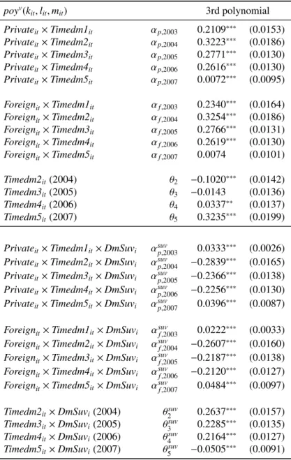
Table 6: Changes in the relative market power of surviving firms poyv(k it, lit, mit) 3rd polynomial Privateit× Timedm1it αp,2003 0.2109∗∗∗ (0.0153) Privateit× Timedm2it αp,2004 0.3223∗∗∗ (0.0186) Privateit× Timedm3it αp,2005 0.2771∗∗∗ (0.0130) Privateit× Timedm4it αp,2006 0.2616∗∗∗ (0.0130) Privateit× Timedm5it αp,2007 0.0072∗∗∗ (0.0095) Foreignit× Timedm1it αf,2003 0.2340∗∗∗ (0.0164) Foreignit× Timedm2it αf,2004 0.3254∗∗∗ (0.0186) Foreignit× Timedm3it αf,2005 0.2766∗∗∗ (0.0131) Foreignit× Timedm4it αf,2006 0.2619∗∗∗ (0.0130) Foreignit× Timedm5it αf,2007 0.0074 (0.0101) Timedm2it(2004) θ2 −0.1020∗∗∗ (0.0142) Timedm3it(2005) θ3 −0.0143 (0.0136) Timedm4it(2006) θ4 0.0337∗∗ (0.0137) Timedm5it(2007) θ5 0.3235∗∗∗ (0.0199)
Privateit× Timedm1it× DmSuvi αsuvp,2003 0.0333∗∗∗ (0.0026) Privateit× Timedm2it× DmSuvi αsuvp,2004 −0.2839∗∗∗ (0.0165) Privateit× Timedm3it× DmSuvi αsuvp,2005 −0.2366∗∗∗ (0.0138) Privateit× Timedm4it× DmSuvi αsuvp,2006 −0.2256∗∗∗ (0.0130) Privateit× Timedm5it× DmSuvi αsuvp,2007 0.0396∗∗∗ (0.0087) Foreignit× Timedm1it× DmSuvi αsuvf,2003 0.0222∗∗∗ (0.0033) Foreignit× Timedm2it× DmSuvi αsuvf,2004 −0.2607∗∗∗ (0.0160) Foreignit× Timedm3it× DmSuvi αsuvf,2005 −0.2187∗∗∗ (0.0138) Foreignit× Timedm4it× DmSuvi αsuvf,2006 −0.2120∗∗∗ (0.0127) Foreignit× Timedm5it× DmSuvi αsuvf,2007 0.0484∗∗∗ (0.0097) Timedm2it× DmSuvi(2004) θ2suv 0.2637∗∗∗ (0.0157) Timedm3it× DmSuvi(2005) θ3suv 0.2285∗∗∗ (0.0135) Timedm4it× DmSuvi(2006) θ4suv 0.2164∗∗∗ (0.0127) Timedm5it× DmSuvi(2007) θ5suv −0.0505∗∗∗ (0.0091)
Equation (12) is used for the estimation. The asterisks∗,∗∗, and∗∗∗ denote 10%, 5%, and 1% significance levels. Figures in parenthe-ses are standard errors, clustered at the 2-digit industrial classifica-tion. poyv(k
it, lit, mit) is approximated by using third order
Figure 1: Changes in the relative markups
Notes: The vertical axis depicts the estimated relative markups for the State, Private+,
and Foreign sectors. The diamond plots and bars indicate the point estimates and the 95% confidence intervals. The relative markups capture a distance from the reference constant term (¯c= c − α0). The term ¯c includesα0indicating the absolute value of markups for the
State sector in 2003. But we cannot identify it in the regression, implying that the absolute
values of markups cannot be measured. To plot the relative markups, the constant term is conveniently normalized at zero by the author.
Figure 2: Changes in the relative markups of surviving firms during the period 2003–2007 Notes: The vertical axis depicts the estimated relative markups of surviving firms in the
State, Private+, and Foreign sectors. The diamond plots and bars indicate the point
esti-mates and the 95% confidence intervals. The relative markups capture a distance from the reference constant term (¯c= c − α0). The term ¯c includesα0indicating the absolute value
of markups for the State sector in 2003. But we cannot identify it in the regression, imply-ing that the absolute values of markups cannot be measured. To plot the relative markups, the constant term is conveniently normalized at zero by the author.
Appendix Table 1: China’s 2-digit Industrial Classification
# Description
13 Agriculture and food processing industry 14 Foodstuff manufacturing industry 15 Soft drink manufacturing industry 17 Textile industry
18 Weaving costume, shoes and cap manufacturing industry 19 Leather, fur and feather manufacturing industry
20 Wood working and wood,bamboo,bush rope,palm,straw manufacturing industry 21 Furniture manufacturing industry
22 Paper making and paper products industry 23 Print and copy of record vehicle industry
24 Stationary and sporting goods manufacturing industry 25 Oil processing, coking and nuclear manufacturing industry 26 Chemical material and chemical product manufacturing industry 27 Medicine manufacturing industry
28 Chemical fiber manufacturing industry 29 Rubber product industry
30 Plastics product industry
31 Nonmetallic mineral product industry
32 Ferrous metal refining and calendaring processing industry 33 Non-ferrous metal refining and calendaring processing industry 34 Metal product industry
35 Universal equipment manufacturing industry 36 Task equipment manufacturing industry
37 Transport and communication facilities manufacturing industry 39 Electric machine and fittings manufacturing industry
40 Communication apparatus, computer and other electric installation manufacturing industry 41 Instrument and meter, stationery machine manufacturing industry
42 Handicraft and other manufacturing industry
Appendix Table 2: Market shares of five largest firms
Notes: Outliers are excluded. The market shares are measured by the fraction of total output by five
Appendix Table 3: Herfindahl-Hirschman Index
Notes: Outliers are excluded. The HHI is measured as the sum of the squares of the firms’ market
Appendix Table 4: Number of firms
Notes: Outliers are excluded. State denotes the set of owned firms, including
state-owned enterprises and solely state-funded corporations. Private+ denotes the set of do-mestic and non-state-owned firms, including collective-owned firms (and other hybrids) and privately funded enterprises. Foreign denotes the set of firms with funds from Hong Kong, Macao, and Taiwan and those that are purely foreign-funded enterprises.
Appendix Table 5: Estimation results with the collectively owned firms dummy vari-ables
(1) (2) (3)
poyv(kit, lit, mit) 3rd polynomial1) 2nd polynomial2) 1st polynomial3)
Collectiveit αc 0.1739∗∗∗ (0.0101) 0.2030∗∗∗ (0.0115) 0.1184∗∗∗ (0.0115) Private∗it αp 0.1793∗∗∗ (0.0103) 0.2095∗∗∗ (0.0116) 0.1217∗∗∗ (0.0110) Foreignit αf 0.1864∗∗∗ (0.0102) 0.2127∗∗∗ (0.0115) 0.1312∗∗∗ (0.0124) Expdmit βex 0.0029∗ (0.0017) 0.0016 (0.0019) 0.0073∗∗ (0.0027) Sizedm2it(2nd Quintile) γ2 0.2815∗∗∗ (0.0093) 0.2635∗∗∗ (0.0102) 0.2357∗∗∗ (0.0083) Sizedm3it(3rd Quintile) γ3 0.4886∗∗∗ (0.0155) 0.4389∗∗∗ (0.0175) 0.4208∗∗∗ (0.0138) Sizedm4it(4th Quintile) γ4 0.7082∗∗∗ (0.0218) 0.6141∗∗∗ (0.0238) 0.6305∗∗∗ (0.0203) Sizedm5it(5th Quintile) γ5 1.0027∗∗∗ (0.0294) 0.8471∗∗∗ (0.0286) 1.0174∗∗∗ (0.0326) Timedm2it(2004) θ2 −0.0177∗∗∗ (0.0049) −0.0105∗∗ (0.0047) −0.0156∗∗∗ (0.0051) Timedm3it(2005) θ3 0.0305∗∗∗ (0.0063) 0.0315∗∗∗ (0.0057) 0.0314∗∗∗ (0.0063) Timedm4it(2006) θ4 0.0628∗∗∗ (0.0083) 0.0613∗∗∗ (0.0075) 0.0701∗∗∗ (0.0084) Timedm5it(2007) θ5 0.0991∗∗∗ (0.0102) 0.0939∗∗∗ (0.0088) 0.1095∗∗∗ (0.0102)
3-digit industrial dummies Yes Yes Yes Province dummies Yes Yes Yes Sample size 1,222,711 1,222,711 1,222,711 Wald tests αp= αf 15.64∗∗∗ 2.77 11.96∗∗∗ αp= αc 11.17∗∗∗ 15.42∗∗∗ 3.13∗ αf = αc 93.52∗∗∗ 51.20∗∗∗ 22.35∗∗∗ γ2= γ3 146.44∗∗∗ 138.53∗∗∗ 138.85∗∗∗ γ3= γ4 130.94∗∗∗ 142.26∗∗∗ 172.40∗∗∗ γ4= γ5 157.95∗∗∗ 166.44∗∗∗ 175.93∗∗∗ θ2= θ3 1007.68∗∗∗ 523.55∗∗∗ 944.84∗∗∗ θ3= θ4 955.33∗∗∗ 699.62∗∗∗ 865.15∗∗∗ θ4= θ5 947.92∗∗∗ 1454.48∗∗∗ 820.80∗∗∗
The asterisks∗,∗∗, and∗∗∗denote 10%, 5%, and 1% significance levels. Figures in parentheses are standard errors, clustered at the 2-digit industrial classification.
1)–3)poyv(k
it, lit, mit) is approximated by using third, second, and first order polynomial series,
respec-tively. Collectiveitdenotes the set of collective-owned firms (and other hybrids). Private∗ denotes
Appendix Table 6: Changes in the relative market power with the collectively owned firm dummy variables
(1) (2) (3)
polyv(kit, lit, mit) 3rd polynomial1) 2nd polynomial2) 1st polynomial3)
Collectiveit× Timedm1it αc,2003 0.2126∗∗∗ (0.0153) 0.2375∗∗∗ (0.0162) 0.1627∗∗∗ (0.0144) Collectiveit× Timedm2it αc,2004 0.2173∗∗∗ (0.0131) 0.2625∗∗∗ (0.0142) 0.1483∗∗∗ (0.0134) Collectiveit× Timedm3it αc,2005 0.1703∗∗∗ (0.0084) 0.1985∗∗∗ (0.0104) 0.1168∗∗∗ (0.0121) Collectiveit× Timedm4it αc,2006 0.1477∗∗∗ (0.0088) 0.1730∗∗∗ (0.0108) 0.0940∗∗∗ (0.0125) Collectiveit× Timedm5it αc,2007 0.0387∗∗∗ (0.0077) 0.0470∗∗∗ (0.0094) −0.0127 (0.0110) Private∗it× Timedm1it αp,2003 0.2313∗∗∗ (0.0157) 0.2581∗∗∗ (0.0164) 0.1735∗∗∗ (0.0139) Private∗it× Timedm2it αp,2004 0.2222∗∗∗ (0.0139) 0.2676∗∗∗ (0.0149) 0.1541∗∗∗ (0.0129) Private∗it× Timedm3it αp,2005 0.1700∗∗∗ (0.0083) 0.1985∗∗∗ (0.0104) 0.1160∗∗∗ (0.0115) Private∗it× Timedm4it αp,2006 0.1511∗∗∗ (0.0080) 0.1773∗∗∗ (0.0099) 0.0956∗∗∗ (0.0119) Private∗it× Timedm5it αp,2007 0.0381∗∗∗ (0.0078) 0.0475∗∗∗ (0.0095) −0.0119 (0.0107) Foreignit× Timedm1it αf,2003 0.2455∗∗∗ (0.0162) 0.2693∗∗∗ (0.0168) 0.1864∗∗∗ (0.0152) Foreignit× Timedm2it αf,2004 0.2337∗∗∗ (0.0141) 0.2774∗∗∗ (0.0151) 0.1679∗∗∗ (0.0138) Foreignit× Timedm3it αf,2005 0.1770∗∗∗ (0.0083) 0.2017∗∗∗ (0.0102) 0.1243∗∗∗ (0.0128) Foreignit× Timedm4it αf,2006 0.1558∗∗∗ (0.0079) 0.1768∗∗∗ (0.0098) 0.1019∗∗∗ (0.0134) Foreignit× Timedm5it αf,2007 0.0405∗∗∗ (0.0078) 0.0455∗∗∗ (0.0096) −0.0030 (0.0127) Timedm2it(2004) θ2 −0.0124 (0.0103) −0.0234∗∗ (0.0094) −0.00002 (0.0079) Timedm3it(2005) θ3 0.0861∗∗∗ (0.0118) 0.0855∗∗∗ (0.0110) 0.0838∗∗∗ (0.0101) Timedm4it(2006) θ4 0.1377∗∗∗ (0.0123) 0.1372∗∗∗ (0.0121) 0.1431∗∗∗ (0.0118) Timedm5it(2007) θ5 0.2854∗∗∗ (0.0163) 0.2976∗∗∗ (0.0159) 0.2876∗∗∗ (0.0167) Wald test αc,2003= αc,2004 0.28 8.83∗∗∗ 3.04∗ αc,2004= αc,2005 27.31∗∗∗ 52.48∗∗∗ 22.42∗∗∗ αc,2005= αc,2006 19.1∗∗∗ 23.37∗∗∗ 17.34∗∗∗ αc,2006= αc,2007 228.65∗∗∗ 165.03∗∗∗ 118.67∗∗∗ αp,2003= αp,2004 1.19 1.61 8.00∗∗∗ αp,2004= αp,2005 34.02∗∗∗ 64.04∗∗∗ 35.27∗∗∗ αp,2005= αp,2006 15.92∗∗∗ 19.24∗∗∗ 15.68∗∗∗ αp,2006= αp,2007 233.04∗∗∗ 163.16∗∗∗ 134.25∗∗∗ αf,2003= αf,2004 2.00 1.21 8.00∗∗∗ αf,2004= αf,2005 34.00∗∗∗ 66.13∗∗∗ 37.47∗∗∗ αf,2005= αf,2006 22.98∗∗∗ 26.41∗∗∗ 19.02∗∗∗ αf,2006= αf,2007 233.41∗∗∗ 167.44∗∗∗ 136.07∗∗∗ θ2004= θ2005 95.56∗∗∗ 119.24∗∗∗ 127.50∗∗∗ θ2005= θ2006 197.90∗∗∗ 153.77∗∗∗ 142.37∗∗∗ θ2006= θ2007 391.23∗∗∗ 256.53∗∗∗ 229.97∗∗∗
The asterisks∗,∗∗, and∗∗∗denote 10%, 5%, and 1% significance levels. Figures in parentheses are standard errors, clustered at the 2-digit industrial classification.
1)–3)poyv(k
it, lit, mit) is approximated by using third, second, and first order polynomial series,
respec-tively. Collectiveitdenotes the set of collective-owned firms (and other hybrids). Private∗ denotes the