On
some
numerical
computations
to
the
oil-reservoir
problems
Tatsuyuki Nakah $\dagger$
($\Psi$
X
$\leqq\not\equiv$) Department of Mathematics,Fukuoka University ofEducation
1. Introduction.
In order to recover part of the remaining oil fiom wells (called production wells), it is
used the way that one injects water into another wells (cffied injection wells), which are
located around the reservoir, so that the water pushes the oil toward the production wells.
In this process, two immiscible fluids
–water and oil –flow through the
porous medium, and can be regarded
as separated by a sharp interface
dur-ing penetration of water into oil. By
Iaboratory
studies,it is already known $r\iota cu*\iota 3l$ $Displ\infty nent$front foramobilityratio$of20$.
showing$thl$$d\cdot v\cdot lopme\mathfrak{n}($of$\Phi\iota\iota e\iota s(alWT\epsilon\pi yuaI.1958)$
.
that the interface is unstable; small
perturbations in the interface
grow
up Fig. 1. Instability of the interface [10].(see Fig. 1).
In this paper we show some numerical computations oftwo-dimensional problems in the
following cases.
Case (a). The water is injected into the injection wells;
Case (b). The pressure given at the injection wells is negative.
The oil-recovery problem stated above corresponds to Case (a). When the capillary
pres-sure between two fluid can be negected, many numerical simulations are done in $[4]-[7]$
and [11]. From the analytical points of view, Chorin [2] proves under some special initial
and boundary conditions that the interface is linearly unstable if$\mu=\mu_{0}/\mu_{w}>3$ and is
lin-early stable if$\mu<3$, where $\mu_{w}$ and $\mu_{0}$ are the viscosities of water and oil, respectively. To
investigate the role of the capillary pressure, we shall show some numerical computations
when the capillary pressure is not neglected.
In Case (b), there exists a steady state solution in one-dimensional problems, and the
numerical
simulationsuggestsusthat this steady statesolution seems tobe stable [8]. Herethe steady state solution means the solution which is independent of time $t$
.
Using thissolution, we can construct a planar wave solution (see (13)) in a rectangle region. We try
to investigate the relationship between the stability of the planar wave solution and the
aspect ratio of the
rectange
region from numerical points of view. The motivation to thisstudy is as follows. In an$otIner$ problems described by some reaction-diffusion equations,
it is already proved that the steady state solution of planar type is stable (resp. unstable)
when the aspect ratio of a rectangle region is small (resp. large). Our aim is to discuss
whether or not the same property holds in the oil-reservoir problems.
In the $fo\mathbb{I}owing$ section, we show the basic equation and the boundary conditions of our
problems. In Section 3, we treat Case (a) from numerical points of view. Some numerical
computations in Case (b) are shown in Section 4.
Thenumerical computations in this paper
are
made by computers FX/1 and FX/4 inDe-partment ofMathematics, Hiroshima University and workstation $Sun4/490$ in Information
Processing Center, Fukuoka University of Education.
2. Basic
equations.
We write water and oil
as
fluid $w$ and fluid $0$, respectively. Let the saturation $s_{i}(x,t)$ be thefractional
amount of fluid $i(i=w, 0)$ at point $x$ and time $t$.
We denote by $v_{i}(x, t)$ and$pi(x, t)$ the velocity and the pressure offluid $i$, respectively. Then we have
1
$s_{w}+s_{o}=1$, (.1)
$- \nabla\cdot\rho|v;=\frac{\partial}{\partial t}(n\rho i^{S_{*})},$ $i=w,$$0$, (2)
$v_{i}=- \frac{Kk_{i}}{\mu:}(\nabla pi-\beta ig)$, $i=w,$$0$, (3)
$p_{0}-p_{w}=p_{c}$
.
(4)Here $\rho i$ and $\mu$; are the density and viscosity offluid $i(i=w, 0),$ $n$ and $K$ are the porosity
and absolute permeability of the medium, and $g$ is the gavity constant. $k_{w}=k_{w}(s_{o})$ and
$k_{o}=k_{o}(s_{w})$ are the relative permeabilities of fluid $w$ and $0$, respectively, and $p_{c}=p_{c}(s_{w})$ is the capillary pressure between two fluids. The forms of these three functions are given
by experiments (see [3], for example), and we take
where $\epsilon$ is some parameter, which means the magnitude of the capillary pressure. The
equation (2) expresses the conservation of fluid $i,$ (3) is Darcy’s law, which means the flow
of fluid $i$ is proportional to the gradient of its pressure. The equation (4) describes the
balance law of the pressure.
For simplicity, we assume that $\rho;,$ $\mu i(i=w, 0),$ $n$ and $K$ are constants with respect to $x$
and $t$, and that there is no external force, that is $g=0$
.
Putting$s=s_{w},$ $v=v_{w}+v_{o}$ and $p=p_{w}$, we can rewrite (1)$-(4)$ as follows.
$\frac{\partial}{\partial t}s+\nabla\cdot[vf(s)]-\epsilon\nabla\cdot[d(s)\nabla s]=0$, (6) $\nabla\cdot v=0$, (7) $v=-[\lambda(s)\nabla p-\epsilon\phi(s)\nabla s]$, (8) where $f(s)= \frac{k_{w}(1-s)}{s)=f(s)\lambda(s)},\lambda(s)=k_{w}(1-s)+\frac,\mu=\frac{\mu_{0}}{\mu_{w}’}d(\phi(s)and\phi(s)=-\frac{k_{o}(s)k_{o}(s)\mu}{\epsilon\mu}p_{c}’(s)$ .
We consider the two-dimensional problem for (6)$-(8)$on$x\equiv(x, y)\in\Omega(l)\equiv(0,1)\cross(0, l)$,
where $\ell$ is positive parameter. Taking Fig.
1 into considerations, we impose the boundary
conditions
$s(0, y, t)=1$, $p(0, y,t)=p^{*}$ on $0<y<\ell$, $t>0$, (9)
$s(1, y,t)=0$, $p(1, y, t)=0$ on $0<y<\ell$, $t>0$, (10)
$\frac{\partial}{\partial y}s(x, y, t)=\frac{\partial}{\partial y}p(x, y,t)=0$ on $(x, y)\in(0,1)\cross\{0,1\}$, $t>0$. (11)
The initial condition
$s(x, y, 0)=s_{0}(x, y)$ on $(x, y)\in\Omega(\ell)$ (12)
is also imposed. The conditions (9)$-(10)$ describe theinjection of water at $\{0\}\cross(0, l)$ with
the pressure $p^{*}$, and the production of oil at
{1}
$\cross(0, \ell)$, respectively. (11) shows that$(0,1)\cross\{0\}$ and $(0,1)\cross\{1\}$ are the Neumann boundaries.
REMARK
1.
Cases (a) and $(b)$.stated in Section 1 correspond to $p^{*}>0$ and $p^{*}<0$,respectively.
Under the boundary conditions (9)$-(11)$, there is
solutions
$s(x, y, t),$ $v(x, y,t),$ $p(x, y,t)$ofthe following foim:
where $\tilde{s}(x,t),\tilde{v}(x,t)$ and $\tilde{p}(x, t)$ are the solution of one-dimensional problem of (6)$-(8)$.
From one-dimensional version of (7), it follows that $\tilde{v}$ does not depend on
$x$. Using this
fact, we find that $\tilde{s}(x, t)$ and $\tilde{v}(t)$ satisfy
$\tilde{s}_{t}+\tilde{v}f(\tilde{s})_{x}-\epsilon(d(\tilde{s})\tilde{s}_{x})_{x}=0$
$\tilde{v}=(p^{*}-c\epsilon)(\int_{0}^{1}\frac{dx}{\lambda(\tilde{s})}I^{-1}$
$\tilde{s}(0, t)=1$ and $\tilde{s}(1,t)=0$
$\tilde{s}(x, 0)=\tilde{s}_{0}(x)$
on $x\in(0,1)$, $t>0$
,
(14)on $t>0$, (15)
on $t>0$, (16)
on $x\in(O, 1)$, (17)
where $c= \int_{0}^{1}\frac{\phi(\sigma)}{\lambda(\sigma)}d\sigma$ is some positive constant.
REMARK 2. In one-dimensional problem (14)$-(17)$, the unknown value$\tilde{p}$ can be
elimi-nated.
REMARK
3.
The solution of the form (13) is called planar iravesolution or solution ofplanar type.
3. Numerical computations in Case (a).
In this section we review some numerical simulations to the twodimensional problems
in Case (a) (see [8]). Throughout this section we set $p^{*}=1$, and the aspect ratio of the
region $\Omega(\ell)$ is fixed to $l=1$
.
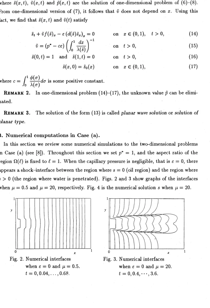
When the capillary pressureis negligible, that is $\epsilon=0$, thereappears ashock-interface between theregion where $s=0$ (oil region) and the region where
$s>0$ (the region where water is penetrated). Figs. 2 and 3 show graphs of the interfaces when $\mu=0.5$ and $\mu=20$, respectively. Fig. 4 is the $niJmerical$ solution $s$ when $\mu=20$.
Fig. 2. Numerical interfaces
when $\epsilon=0$ and $\mu=0.5$
.
Fig. 3.
Numerical
interfaces when $\epsilon=0$ and $\mu=20$.
$t=3.6$
Fig. 4. Numerical simulation when $\epsilon=0$ and $\mu=20$.
From these figures, one can find that the interface seems to be stable when $\mu=0.5$.
However, when $\mu=20$, the interface is unstable. In one-dimensionaJ problems, we already
know the following theorem.
TIIEOREM 4.[8] Let $t\Lambda e$ initiaI function be $\tilde{s}_{0}\equiv 0$. $T\Lambda ent\Lambda e$ interface $\eta(t)$ of the
solution of (14)$-(17)$ satisfies
$\eta’’(t)<0$ on $0<t<T_{b}$ i$f$ $0<\mu<\mu^{*}$, (18)
$\eta’’(t)>0$ on $0<t<T_{b}$ if $\mu>\mu^{*}$, (19)
1
$w\Lambda ereT_{b}$ is some positi$ve$ constant satisfying$\eta(T_{b})=1$, and $\mu^{*}=1.65\cdots$
.
REMARK
5.
The constant $T_{b}$ in the previous theorem is called the $breaktInioug\Lambda$ time,which means the time when water reaches to the production wells.
To investigate the role of the capillary pressure, let us consider the case of $\epsilon>0$. In the following we set $\mu=20$; the case where the interface is unstable when $\epsilon=0$
.
For small value of$\epsilon$, the interface is also unstable (see Fig. 5).$t=3.6$
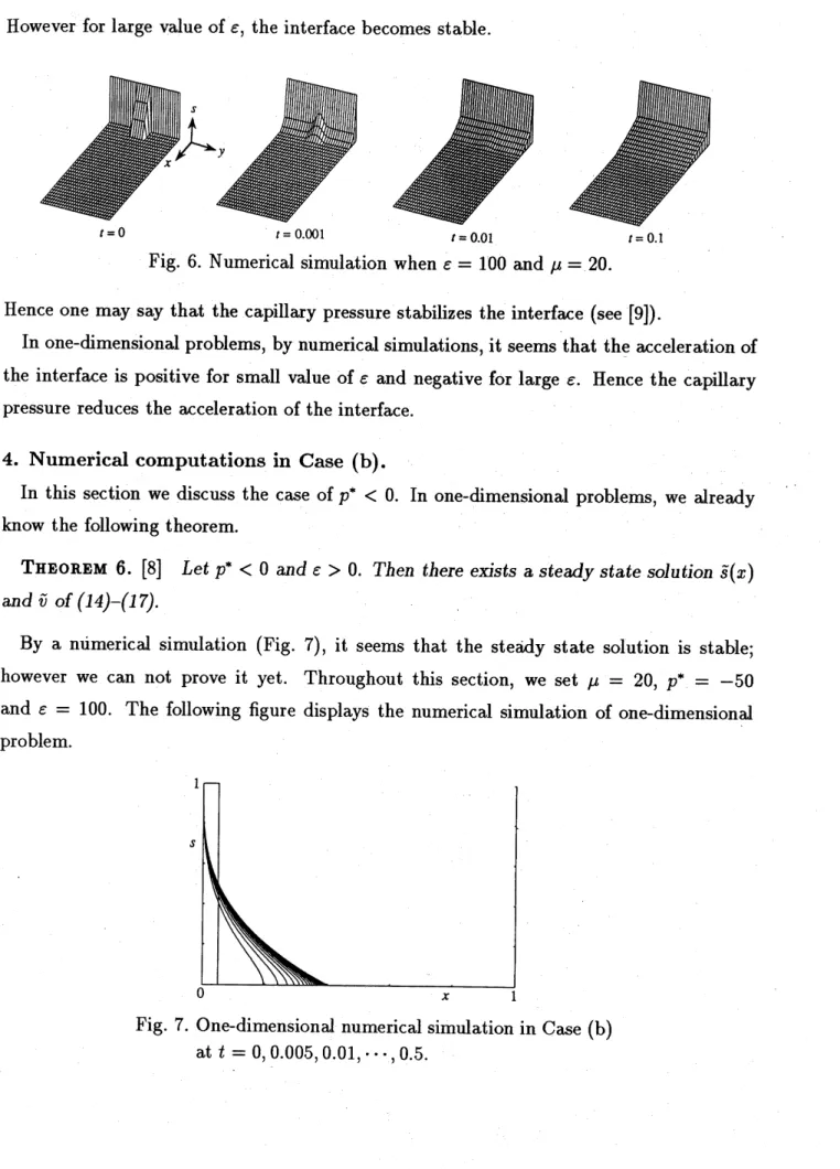
However for large value of$\epsilon$, the interface becomes stable.
$t=0.01$
Fig. 6. Numerical simulation when $e=100$ and $\mu=20$
.
Hence one may say that the capillary pressure stabilizes the interface (see [9]).
In one-dimensional problems, by numerical simulations,it seemsthat the accelerationof
the interface is positive for small value of$\epsilon$ and negative for large
$\epsilon$
.
Hence the capillarypressure reduces the acceleration ofthe interface.
4. Numerical computations
in
Case (b).In this section we discuss the case of$p^{*}<0$
.
In one-dimensional problems, we alreadyknow the following theorem.
TIIEOREM
6.
[8] Let $p^{*}<0$ and $\epsilon>0$.
Then there exists a $steadystate$ solution $\tilde{s}(x)$ and $\tilde{v}$ of (14)$-(17)$.
By a numerical simulation (Fig. 7), it seems that the steady state solution is stable;
however we can not prove it yet. Throughout this section, we set $\mu=20,$ $p^{*}=-50$
and $\epsilon=100$
.
The following figure displays the numerical simulation of one-dimensionalproblem.
Fig. 7.
One-dimensional
numerical simulationin Case (b)By simple calculations, we find that the steady state
solution
$\tilde{s}(x)$ satisfies$\tilde{s}(x)=\{\begin{array}{ll}1-(x/\eta)^{1/3}, if 0\leq x\leq\eta,0, if \eta<x\leq 1,\end{array}$ (20)
where $\eta=0.4$is the position of the interface. Let us construct the two-dimensional steady
state solution of planar type by (13), and we investigate the stability of this solution from
numerical points of view. We take the initial function $s_{0}(x, y)$ as
$s_{0}(x, y)=\{\begin{array}{ll}1-(x/\eta(y))^{1/3}, if 0\leq x\leq\eta(y), 0\leq y\leq l,0, if \eta(y)<x\leq 1, 0\leq y\leq l,\end{array}$ (21)
where $\eta(y)=0.4+0.2\cos\frac{\pi}{\ell}y$
.
The following figure demonstrates numerical simulation when $f=0.01$.
Fig. 8. Numerical simulation in Case (b) when $\ell=0.01$
.
One can see that the steady state solution ofplanar type is stable in this case.
Next we show $tbe$ case where $\ell=1000$
.
$t=0$ $t=0.\infty 5$ $t=0.015$ $t=0.05$ Fig. 9. Numerical simulation in Case $($b) when $\ell=1000$.
In this
case
the steady statesolution
of planar type also seems to be stable. We carry oncomputations when $\ell=0.1,1,10,100$
.
In all cases, we observe that the solutions seem toReferences.
[1] J.Bear, Dynamics of Fluids in Porous Media, American Elsevier Publishing Company
Inc., 1972.
[2] A.J.Chorin, The instability offronts in a porous medium, Comm. Math. Phys., 91
(1983), 103-116.
[3] L.P.Duke, Fundamentals ofReservoirEngineering, Elsevier Science Publishing
Com-pany Inc., 1978.
[4] R.E.Ewing, The Mathematics of Reservoir Simulations, SIAM, 1983.
[5] W.E.Futzgibbon, Mathematical and Computational Methodsin Seismic Exploration
and Reservoir Modeling, SIAM, 1986.
[6] J.Glimm, D.Marchesin and O.McBryan, Unstable fingers in two phase flow, Comm.
Pure Appl. Math., 24 (1981), 53-75.
[7] P.R.King, The Mathematics of Oil Recovery, Clarendon Press, 1992.
[8] T.Nakaki, Numerical treatment on the behavior of interfaces in oil-reservoir
prob-lems, Hiroshima Math. J., 23 (1993), 417-448.
[9] T.Ohta, Butsurigaku saizensen, 10 (1985), 3-69, Ky\^oritsu shuppan (in Japanese).
[10] A.E.Scheidegger, The Physics of Flow Through Porous Media, Third edition,
Uni-versity of Toronto Press, 1974.