A method of computations of fundamental groups of 3-dimensional manifolds (Fundamental Groups and Algebraic Functions)

(1)

A method

of computations of

fundamental groups

of

3-dimensional manifolds

Maki Takai

(

高井

真希

)

1 Introduction.

By the theorem of Hilden-Montesinos (Hilden [7], Montesinos [9]), for every

3-dimensional compact oriented manifold$\mathrm{Y}$, there exists a topological branched

cov-ering

$h$

:

$\mathrm{Y}arrow S^{3}$

of the 3-sphere $S^{3}$ of degree 3 branching at a knot $B_{h}$, whose monodromy around

the knot is given only by transpositions.

We regard the knot $B_{h}$ as abraid, for every knot (and link) is isotopic in $S^{3}$ to

a braid. We may identify $S^{3}$ with $\partial(\overline{\Delta(\mathrm{o},a^{;})}\cross\Delta(\mathrm{O}, b’))$, where

$\Delta(0, a’)$ is the disc

in the complex plane $\mathbb{C}$ with the center $0$ and the radius $a’$

.

We may assume that

$B_{h}$ is contained in $\partial\overline{\Delta(0,a^{J})}\cross\Delta(0, b^{l})$ as in Figure 1.

$(0\leq s\leq 2\pi)$

Figure 1:

Let $B$ be

$\mathrm{t}.\mathrm{h}.\mathrm{e}$ cone over

$B_{h}$

conneCtin.g

every

$.\mathrm{p}$oint of

$B_{h}$ with the origin of $\mathbb{C}^{2}$

.

Let

$f$ : $Xarrow\Delta(\mathrm{O}, a)\cross\Delta(0, b)$

be thetopological finite branched covering branching at $B\mathrm{w}\mathrm{i}\mathrm{t}\mathrm{h}’ \mathrm{t}\mathrm{h}\mathrm{e}$ samemonodromy

(2)

cone over Y.) Since $X$ is a topological cone

over

$\mathrm{Y}$,

$\pi_{1}(X-\{_{X}\}, p_{0})\simeq\pi_{1}(\mathrm{Y}, p0)$, $(x=f^{-1}((0,0)))$

.

Put

$X_{t}$ $=f^{-1}(t\mathrm{X}\Delta(0, b))$,

$f_{t}$ $=f|_{X_{t}}$

:

$X_{t}arrow t\mathrm{x}\Delta(0, b)$

.

Then every $f_{t}(t\neq 0)$ is a finite branched covering of the disc $t\cross\Delta(\mathrm{O}, b)$

,

and

$f$ can be regarded as a topological degenerating family offinite branched coverings

of discs: $f=\{f_{t}\}$

.

Its topological type is determined by the pair

$(\Phi_{t}, \theta(\delta))$, $(\delta:s\mapsto a’e^{is}, (0\leq S\leq 2\pi))$

of the monodromy $\Phi_{t}$ of $f_{t}$ (for a fixed $t\neq 0$) and the braid monodromy $\theta(\delta)$ of$f$

.

But they must $\mathrm{S}\mathrm{a}\mathrm{t}\mathrm{i}\mathrm{s}\mathfrak{h}^{r}$ the following equality (Namba [10]):

$\Phi_{t}0\theta(\delta)=\Phi t$,

where $\theta(\delta)$ is regarded as an automorphism of $\pi_{1}(t\cross\Delta(\mathrm{o}, b)-B_{f,q0})$ (see Section

2).

Conversely, let

$\Phi$ : _{$\pi_{1}(\Delta(0, b)-$}

{

$n$ points}, $q\mathrm{o})arrow S_{d}$

be a representation whose image is a transitive subgroup of the d-th symmetric

group $S_{d}$

.

Let $\sigma$ be a braid which satisfies

$\Phi\circ\sigma=\Phi$

.

We denote the $n$-pointsby $\{q_{1}, \ldots , q_{n}\}$ and let $\gamma_{1},$ $\ldots$

,

$\gamma_{n}$ bethelassos as inFigure

2.

Then

$\pi_{1}(\Delta(\mathrm{o}, b)-\{q_{1}, \ldots, qn\},$ $q0)=<\gamma 1,$ _$\ldots,$ $\gamma_{n}>$

is a free group. Put

$A_{j}=\Phi(\gamma_{j})$ $(j=1,2, \ldots, n)$

.

We regard the braid $\sigma$ as a link which is contained in

$\partial\overline{\Delta(\mathrm{o},a’)}\mathrm{X}\Delta(0, b’)$ as

in Figure 1. By the condition $\Phi 0\sigma=\Phi$, we can construct a topological branched

covering

$h$ : $\mathrm{Y}arrow\partial(\overline{\Delta(0,a’)}\cross\overline{\Delta(\mathrm{o},b’)})$

branching at the link $\sigma$ whose monodromy is $\Phi$

.

More precisely, we can construct

a topological branched covering $\mathrm{Y}’$ of $\partial\overline{\Delta(0,a)\prime}\cross\Delta(\mathrm{O}, b’)$ branching at the link $\sigma$

whose monodromy is $\Phi$

.

We then attach solid tori to $\mathrm{Y}’$ at the part corresponding

to the mutually prime cyclic decomposition of the permutation

(3)

$q_{0}$

Figure 2:

over $\partial\overline{\Delta(0,a)\prime}\cross\partial\overline{\Delta(0,b’)}$

.

Then we get a 3-dimensional compact oriented manifold $\mathrm{Y}$ and a topological finite branched covering

$h$ : $\mathrm{Y}arrow\partial(\overline{\Delta(0,a’)}\cross\overline{\Delta(\mathrm{o},b\prime)})$

of the 3-sphere branching at the link a whose monodromy is $\Phi$

.

We then construct the topological cone $X$ of$\mathrm{Y}$ as above and construct a

topo-logical finite branched covering

$f$ :$Xarrow\Delta(\mathrm{o}, a)\mathrm{x}\Delta(\mathrm{o}, b)$

such that

$\Phi_{f}=\Phi$, $\theta(\delta)=\sigma$

.

This isregarded asa topological degeneratingfamily of finitebranched coverings of discs.

Thus to construct topological degenerating families of finite branched covering$s$

of discs (hence to construct 3-dimensional compact oriented manifolds) is reduced

to find out the pair $(\Phi, \sigma)$ as above such that $\Phi 0\sigma=\Phi$

.

2 Monodromy of

a

branched

covering

of

degree

3 of the disc and

its

canonical forms.

Let $X$and $\mathrm{Y}$ beRiemann surfaces and let

$f$ : $Xarrow \mathrm{Y}$beafinite branched covering,

that is, a surjective proper finite holomorphic mapping. A point $p$ of$X$ is called a

ramification point of $f$ if $f$ is not biholomorphic around $p$

.

Its image $q=f(p)$ is

called a branch point of$f$

.

The set of all ramification points (resp. branch points) is

denoted by $R_{f}$ (resp. $B_{f}$ ) and is called the ramification locus (resp. branch locus).

Then

(4)

is an unbranched covering, whose mapping degree is called the degree of $f$ and is

denoted by degf. (X, $f$) (or simply $f$) is called a finite branched covering of Y.

Deflnition 1. Two

_finite

branched coverings

$f:Xarrow \mathrm{Y}$, $f’:x’arrow \mathrm{Y}$

are said to be isomorphic

_if

there is a biholomorphic mapping $\psi$ which makes the

following diagram commutative:

.

$X \frac{\psi\backslash }{r}X’$

$f\downarrow$ $\downarrow f’$

$\mathrm{Y}arrow\dot{.}d\mathrm{Y}$

Deflnition 2. Two

_finite

branched coverings

$f:Xarrow \mathrm{Y}$, $f’:X’arrow \mathrm{Y}$

are said to be equivalent (resp. topologically equivalent)

_if

there are biholomorphic

mappings (resp. $or\dot{\eta}entation$ preserving homeomorphisms) $\psi$ and $\varphi$ which make the

following diagram commutative:

$Xarrow\psi X’$

$f\downarrow$ $\downarrow f’$

$\mathrm{Y}arrow^{\varphi}\mathrm{Y}$

Let $B_{n}$ be the Artin braid group of $n$ strings. Then $B_{n}$ is expressed as follows:

$B_{n}=<\sigma_{1},$

$\ldots,$ $\sigma n-1$ $|\sigma_{i}\sigma_{i}+1\sigma*\cdot=\sigma_{i}+1\sigma i\sigma i+1$

$\sigma_{i}\sigma_{j}=\sigma_{j}\sigma_{i}$, for $|i-j|\geq 2>$

.

Let $\{q_{1}, \ldots , q_{n}\}$ be a set of $n$ distinct points in C. The fundamental group $\pi_{1}(\mathbb{C}-\{q_{1}, \ldots , q_{n}\}, q_{0})$ is the free group

$\pi_{1}(\mathbb{C}-\{q1, \ldots, qn\}, q\mathrm{o})=<\gamma_{1},$ _$\ldots,$ $\gamma_{n}>$

generated by the lassos $\gamma_{1},$ _$\ldots,$ $\gamma_{n}$ as in Figure 2.

The braid group $B_{n}$ acts on this group as follows:

$-$ .

$\sigma_{i}(\gamma_{i})$ $=\gamma_{i}^{-1}.\gamma i+1\gamma i$

$\sigma:(\gamma_{i+1})$ $=’\gamma_{i}$

$\sigma_{i}(\gamma_{j})$ _{$=\gamma_{j}$} $(j\neq i, i+1)$

.

Note that this action is faithful (Birman [1]). A similar assertion holds ifwe replace

$\mathbb{C}$ by adisc _{$\Delta(0, b)$}

.

(5)

Theorem 1. Put $B=\{q_{1}, .\mathrm{Y}. , q_{n}\}\subset \mathrm{P}^{1}=\mathbb{C}\cup\{\infty\}$. For any homomorphism

$\Phi:\pi_{1}(\mathrm{P}1-B, q0)arrow S_{d}$ whose image $Im\Phi$ is transitive, there exists a unique (up

to isomorphisms)

_finite

branchedcovering $f$ :$Xarrow \mathrm{P}^{1}$ such that

$B_{f}\subset B$, $\Phi_{f}=\Phi$

.

For theproof ofTheorem1, see Forster [4]. There is a higher dimensional analogy

of the theorem (Grauert-Remmert [6]).

Theorem 2. For two

_finite

branched coverings $f$

:

$Xarrow \mathrm{P}^{1}$, _$f’$ : $X’arrow \mathrm{P}^{1}$ such

that $B_{f}=B_{f’}=\{q_{1}, \ldots , q_{n}\}\subset \mathbb{C}$ , they are topologically equivalent

if

and only

if

there is a braid $\sigma$ in $B_{n}$ such that $\sigma^{*}(\Phi_{f})=\Phi_{f}0\sigma=\Phi_{f’}$. Here the equality is that

as representation classes.

For the proofof Theorem 2, see Namba [10].

Remark. Theorem2 holds even if$\mathrm{P}^{1}$ is replaced by the compelx plane $\mathbb{C}$ or a disc

in C.

Every branched covering

$f$ : $Xarrow\Delta(0, b)$

ofdegree $d$can be extended to a branched covering

$\hat{f}:\hat{X}arrow \mathrm{P}^{1}$

of degree $d$ in the following canonical manner: Put

$B_{f}=\{q_{1}, \ldots, q_{n}\}$, $A_{j}=\Phi_{f}(\gamma_{j})$ $(j=1, \ldots, n)$,

where $\gamma_{j}$ is a lasso as in Figure 2. Let $\gamma_{\infty}$ be the lasso around the point $\infty$ as in

Figure 3.

Then

$\pi_{1}(\mathrm{P}^{1}-\{q1, \ldots, q_{n}, \infty\}, q\mathrm{o})=<\gamma 1,$ _$.:$

.

$,$ $\gamma_{n},$

$\gamma\infty|\gamma_{\infty}\gamma_{n}\cdots\gamma 1=1>$

.

Put

$A_{\infty}=(A_{n}\cdots A_{1})^{-1}$

.

We define a homomorphism

$\Phi:\pi_{1}(^{\mathrm{p}}1-\{q1, \ldots, q_{n}, \infty\}, q0)arrow S_{d}$

by

$\Phi(\gamma_{j})=A_{j}$ $(j=1, \cdots n)$, $\Phi(\gamma_{\infty})=A_{\infty}$

.

Then the branched covering

$\hat{f}:\hat{X}arrow \mathrm{P}^{1}$

(6)

$q_{0}$

Figure 3:

Note that if$A_{\infty}=1$, then $\hat{f}$ does not branch at the point $\infty$

.

Let

$f$

:

$Xarrow\Delta(0, b)$

be a branched covering of the disc $\Delta(0, b)$ ofdegree 3. Let $\gamma_{j}(j=1, \ldots , n)$ be the

lassos as in Figure 2. Put $A_{j}=\Phi_{f}(\gamma_{j})$ ($j=1,$ _$\ldots$ , n). Suppose that every $A_{j}$ is a

transposition in the 3rd symmetric group $S_{3}$

.

As above, we extend the covering to

that of $\mathrm{P}^{1}$ which is denoted by the same notation _$f$ for simplicity. Let

$\gamma_{\infty}$ be the

lasso around the point $\infty$ and put

$A_{\infty}=(A_{n1}\ldots A)^{-}1=\Phi_{f(\gamma)}\infty$

as above. There are three cases:

Case 1. $A_{\infty}=1$

.

In this case, the extended covering does not branch at $\infty$

.

Case 2. $A_{\infty}$ is a transposition. In this case, the point $\infty$ is a branch point, that

is there is a point over $\infty$ with the ramification index is 2. Since we may

change the monodromy with an equivalent representation

,

we may assume

that $A_{\infty}=(12)$

.

Case 3. $A_{\infty}$ is a cyclic permutation. In this case, the point $\infty$ is a branch point.

We may assume that $A_{\infty}=(132)$

.

Under these assumptions, we have the following theorem:

Theorem 3. Underthe above assumptions, the covering$f$ is topologically equivalent

to one

_of

the following canonical

_forms:

Arranging $A_{1},$ $A_{2},$

$\ldots,$ $A_{n}$ in this order:

(7)

Case 2: (12),(23), (23),

where $g\iota s$ the genus

of

the Riemann

surface

$X$

.

3 _{Isotropy subgroups of the braid}

_groups.

Let

$\Phi:<\gamma_{1},$

$\ldots,$ $\gamma_{n}>arrow sd$

be a representation _{of the free} group $<\gamma_{1},$ _$\ldots$

,

$\gamma_{n},>\mathrm{o}\mathrm{f}n$ generators into the d-th

symmetric group $S_{d}$ whose image $Im\Phi$ is transitive.

By the discussion in Section 1, it is important to consider the braid $\sigma\in B_{n}$

such that $\Phi 0\sigma=\Phi$, where the equality is not as representaion _{classes but is just}

as representaions. (The action of the braid $\sigma$ on the free group

$<\gamma_{1},$ $\ldots$

,

$\gamma_{n}>\mathrm{i}\mathrm{s}$

defined in Section 2.) Put

$I(\Phi)=\{\sigma\in B|n\Phi 0\sigma=\Phi\}$,

the isotropy subgroup of $B_{n}$ for $\Phi$

.

Since the number ofrepresentaions $\Phi$ is finite (in fact is less than

$(d!)^{n}$), $I(\Phi)$ is

asubgroup of $B_{n}$ of finite index.

Note that the following equality holds:

$I(\Phi 0\tau)=\tau-1I(\Phi)\tau$

.

Put

$\Phi(\gamma_{j})=A_{j}$ $(j=1,2, \cdots, n)$

.

Now, let $\Phi$ be the representation of the canonical forms as

in Theorem 3.

For Case 2 and 3 $(\mathrm{i}.\mathrm{e}, A_{1}=(12),$ _{$A_{2}=\cdots=A_{n}=(23))$}, by the theorem of

Birman-Wajnryb (Birman-Wajnryb [2]) $I(\Phi)$ is generated by the following elements:

$\sigma_{1}^{3},$

$\sigma_{2}$,

...

,

$\sigma_{n-1}$,

$\sigma_{1}^{-1}\sigma_{2}^{-}\sigma-2\sigma_{2}\mathrm{r}3-1\sigma_{1}-\mathit{2}-\sigma_{2}\iota 1\sigma^{-}3\sigma_{43}\sigma\sigma_{2}\sigma_{1\mathit{2}3}2\sigma\sigma\sigma_{2}2\sigma_{1}(n\geq 5)$

.

The following theorem for Case 1 $(\mathrm{i}.\mathrm{e}, A_{1}=A_{2}=(12),$ _{$A_{3}=\cdots=A_{n}=(23))$}

is the main result.

Theorem 4. For Case 1, $I(\Phi)$ is generated by the following elements:

$\sigma_{1},$ $\sigma_{2}^{3},$ $\sigma_{3}$,

...

,

$\sigma_{n-1},$ $\sigma_{2}^{-1}\sigma_{3}^{-}\sigma_{2}\sigma 2-11\sigma \mathit{2}\sigma 3\mathit{2}\sigma 2$, $\sigma_{2}^{-1}\sigma_{3}^{-}\sigma_{4}\sigma^{-}\sigma_{2}\sigma^{-}\sigma_{4}\sigma 1-231-231-15\sigma 4\sigma_{3}\sigma_{234}\mathit{2}\sigma\sigma\sigma_{3}2\sigma_{2}(n\geq 6)$

.

Remark. For Case 1, the generators ofthe isotropy subgroup $I(\Phi)$ of $B_{n}(S^{\mathit{2}})$ are

(8)

4 Riemann pictures

and symplectic basis

for

canon-ical

forms.

In this section, we introduce a picture, (we call it a Riemann picture), which

repre-sents a finite branched covering of a disc $\mathrm{t}\mathrm{o}\mathrm{p}\mathrm{o}1.\mathrm{o}\mathrm{g}\mathrm{i}_{\mathrm{C}\mathrm{a}}11\mathrm{y}$ (see Namba-Takai [11]). We

explain it by an example:

Let us consider Case 1 ofgenus 1.

Let $X$ be a Riemann surface of genus 1. Let $f$

:

$Xarrow \mathbb{C}$ be a branched

covering of degree 3 with the monodromy $\Phi$ of canonical form of Case 1. Put

$B_{f}=\{q_{1}, q_{2}, \ldots , q_{6}\}$

.

Let $q_{0}$ be a reference point. We take the lassos $\gamma_{j}$ around $q_{j}$

as in Figure2. We extend the coveringto thebranched covering of$\mathrm{P}^{1}$ in a canonical

way as in Section 2. In this case, we have

$\pi_{1}(^{\mathrm{p}_{-}^{1}}B_{f}, q\mathrm{o})=<\gamma_{1},$ $\gamma 2,$ $.,.,$ $\gamma\epsilon,$ $\gamma_{\infty}|\gamma\infty\gamma\epsilon\cdots\gamma 2\gamma 1=1>$,

$A_{1}=A_{2}=(12)$ $A_{\mathit{2}}=\cdots A_{6}=(23)$, $A_{\infty}=id$ $(A_{j}=\Phi(\gamma_{j}))$

.

Consider the picture (Figure 4) in which the circle part of every lasso $\gamma_{j}$ in Figure

2 is degenerated to the point $q_{j}$:

$q_{0}$

Figure 4:

We then pull the picture in Figure 4 backoverthe covering$f$and get the following

picture in Figure 5 which we call the Riemann picture of$f$:

In Figure 5, the point$s$ \copyright, \copyright, \copyright are the inverse images of the reference point

$q_{0}$ while the pointts 1,

...

, 6 and $\infty$ are the inverse images of $q_{1},$ $\ldots$ , $q_{6}$ and $\infty$ respectively. Note that around every point \copyright, \copyright, \copyright, the pathes connecting to the

points 1,

...

,

6 and $\infty$ in this order are arranged clockwisely. On the other hand,

around every point 1,

...

,

6 and $\infty$, the pathes connecting to the points \copyright, \copyright, \copyright

are arranged counterclockwisely in order to be compatible with the monodromy.

(We omit unramified points in the picture.)

The covering (X, $f$) can be topologically expressed by this picture.

Put $\xi_{3}$ _$=$ $[1, 21][\infty, 11][1,12]$, $\xi_{2}$ _$=$ $[\infty, 22]$, . $\xi_{1}$ _$=$ $[6, 23][\infty, 33][6,32]$, $\alpha=$ $[3, 23][4,32]$, $\beta=$ $[5,23][4,32]$

.

(9)

Figure 5:

Here the notation $[6, 23]$ for example

means

the path in Figure 5 whose initial

point is \copyright and the terminal point is \copyright passing through the branch point 6. Then

these are loops with the initial point \copyright. We can observe the following relations:

$\beta\alpha\beta^{-1}\alpha^{-}\xi_{3}1\xi_{2}\xi_{1}$ $=1$,

$<\alpha,$ $\beta>$ $=$ $1$,

where thenotation $<,$ $>\mathrm{m}\mathrm{e}\mathrm{a}\mathrm{n}\mathrm{s}$theintersection number. We pullback the relation

$\gamma_{\infty}\gamma_{6}\cdots\gamma_{1}=1$

over $f$ and get the following three relations:

$[\infty, 11][2,12][1,21]=1$,

$[\infty, 22][6,23][5,32][4,23][3,32][2,21][1,12]=1$, $[\infty, 33][6,32][5,23][4,32][3,23]=1$

.

The above relation

$\beta\alpha\beta^{-1}\alpha^{-}\xi_{3}1\xi 2\xi_{1}=1$

can be induced from these three relations.

The Riemann picture of a general (X, $f$) is definedasin the aboveexample, that

is, a pull-back over $f$ of the graph on $\mathrm{P}^{1}$ of Figure 2 degenerated the

circle part of

every lasso to the branch point.

Remark. 1. The Riemann picture is determined by (X, $f$) up to orientation

preserving homeomorphisms of$X$

.

2. As noted above, we can draw the Riemann picture of (X, $f$) even when only the

monodromy $\Phi=\Phi_{f}$ is given and (X, $f$) is not explicitely given.

(10)

topologically, which we called a Klein picture. Klein pictures and Riemann pictures

aredual in asense. Klein picturesareusefultoobserve the degeneration ofbranched

coverings, while Riemann picutres are usefulto computefundamental groups as will

be seen in Section 5.

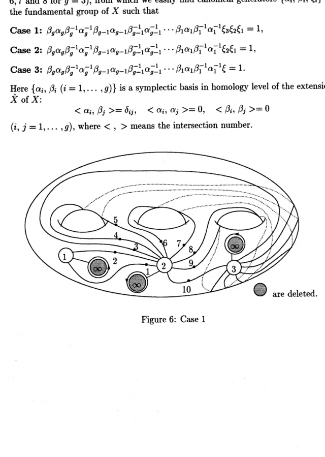
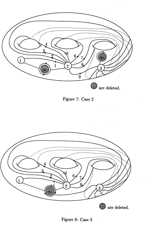
We draw the Riemann pictures of thecanonical forms in Theorem 3 (see Figures

6,7 and 8 for $g=3$), from which we easily find canonical generators $\{\alpha_{i}, \beta i, \xi_{i}\}$ of

the fundamental group of$X$ such that

Case 1: $\beta_{g}\alpha_{g}\beta_{g}^{-1-}\alpha_{g}1\beta g-^{\iota 1\beta_{g}^{-1}\alpha_{g1}^{-}}\alpha g--1-1\ldots\beta 1\alpha_{1}\beta 1-1\alpha_{1}-1\xi 3\xi_{\mathit{2}}\xi_{1}=1$,

Case 2: $\beta_{g}\alpha_{g}\beta^{-1-}gg\alpha 1\beta_{g}-1\alpha g-1\beta_{g-1}^{-1}\alpha_{g1}^{-}-1\ldots\beta 1\alpha_{1}\beta^{-1}11\alpha^{-}1\xi 2\xi_{1}=1$,

Case 3: $\beta_{g}\alpha_{g}\beta_{ggg1}-1-\alpha 1\beta_{g1g-}-\alpha 1\beta_{g-}^{-1}1\alpha--1\ldots\beta_{11}\alpha\beta^{-}11\alpha_{1}^{-}\xi 1=1$

Here $\{\alpha_{i}, \beta_{i} (i=1, \ldots , g)\}$ is a symplectic basis in homology level of the extension

$\hat{X}$

of$X$:

$<\alpha_{i},$ $\beta_{j}>=\delta_{ij}$, $<\alpha_{i},$ $\alpha_{j}>=0$, $<\beta_{i},$ $\beta_{j}>=0$

$(i, j=1, \ldots,g)$, where $<,$ $>\mathrm{m}\mathrm{e}\mathrm{a}\mathrm{n}\mathrm{s}$ the intersection number.

(11)

Figure 7: Case 2

$\bullet$

are deleted.

(12)

In fact we may take as follows: Case 1: $\xi_{3}$ $=$ $[1, 2l][\infty, 11][1,12]$ ’ $\xi_{2}$ $=$ $[\infty, 22]$ . $\xi_{1}$ $=$ $[2g+4,23][\infty, 33][2g+4,32]$ $\alpha_{1}$ $=$ $[3, 23][4,32]$ $\beta_{1}$ $=$ $[5, 23][4,32]$ $\alpha_{j}$ $=-[2j+1,23][2j, 32]\cdots[3,23][2j, +2,32]$ $\beta_{j}$ $=$ $[2j+3,23][2j+2,32]$ $\alpha_{g}$ $=$ $[2g+1,23][2g, 32]\cdots[3,23][2g+2,32]$ $\beta_{\theta}$ $=$ $[2g+3,23][2g+2,32]$

.

Case 2:

$\xi_{\mathit{2}}$ $=$ $[\infty, 21][\infty, 12]$

$\xi_{1}$ $=$ $[2g+3,23][\infty, 33]12g+3,32]$ $\alpha_{1}$ $=$ $[2, 23][3,32]$ $\beta_{1}$ $=$ $[4,23][3,32]$ $\alpha_{j}$ $=$ $[2j, 23][2j-1,32]\cdots[2,23][2j+1,32]$ $\beta_{j}$ $=$ $[2j+2,23][2j+1,32]$ $\alpha_{g}$ $=$ $[2g, 23][2g-1,32]\cdots[2,23][2g+1,32]$ $\beta_{g}$ $=$ $[2g+2,23][2g+1,32]$

.

Case 3:

$\xi$ $=$ $[\infty, 21][\infty, 13][\infty, 32]$

$\alpha_{1}$ $–[2^{:},$ $231[3,32]$ $\beta_{1}$ $=$ $[4, 23]13,32]$ $’\lambda$ $\alpha_{j}$ $=$ $[2j, 23][2j-1,32]\cdots[2,23][2j+1,32]$ $\beta_{j}$ $=$ $[2j+2,23][2j,+1,32]$ $\alpha_{g}$ $=$ $[2g, 23][2g-1,32]\cdots[2,23][2g+1,32]$ $\beta_{g}$ $=$ $[2g+2,23][2g+1,32]$

.

(13)

5Calculations

of

fundamental

groups.

In this section, we compute fundamental groups of 3-dimensional compact oriented

manifolds using the local version of the theorem of Zariski-van Kampen (see Dimca

[3], Matsuno [8]$)$ and the method of Reidemeister-Schreier (see Rolfsen [12]). One

cancomputethe fundamental group rigorously ifone uses the Riemann picture. We

explain this using a concrete example:

Let us

_cons.ider

Case 1 ofgenus 1 for simplicity. Ifwe take the braid $\sigma$ as

$\sigma=\sigma^{-1}\sigma^{-}\sigma^{-}\sigma 1\sigma \mathit{2}\sigma\sigma 23\mathit{2}21\mathit{2}\mathit{2}35\sigma\sigma_{4}\sigma 3\sigma 32$ ($\sigma$ induces a knot), then we have the equality

$\Phi 0\sigma=\Phi$

where $\Phi$ is the monodromy of the canonical form. Hence we may construct a

topo-logical degenerating family

$f$ : $Xarrow\Delta(\mathrm{o}, a)\mathrm{x}\Delta(\mathrm{o}, b)$

ofbranched coverings of discs constructed from the pair $(\Phi, \sigma)$ (see Section 1). Let

$B_{f}$ be the branch locus of$f$. Let $\gamma_{j}$ $(j=1, \ldots , 6)$ be the lassos as in Figure 2. The

local version of the theorem of Zariski-van Kampen asserts that the fundamental

group of$\Delta(0_{\backslash ,J}a)\cross\Delta(\mathrm{O}, b)-B_{f}$ is generated by $\gamma_{j}(j=1, \ldots , 6)$ whose generating

relations are $\sigma(\gamma_{j})=\gamma_{j}(j=1, .., , 6)$

.

That is to say

$\pi_{1}(\triangle(0, a)\cross\Delta(0, b)-B_{f},$ $q\mathrm{o})=<\gamma 1,$$\ldots,\gamma_{6}|\sigma(\gamma j)=\gamma j(j=1, \ldots, 6)>$

$=<\gamma_{1},$

$\ldots,\gamma_{6}|(\sigma_{232}-12-1\sigma\sigma^{-}\sigma\sigma_{1}\sigma 23\sigma 2\sigma-1-125\sigma_{4}\sigma 3\sigma^{3})2\gamma_{j\gamma_{j}}=(j=1, \ldots,6)>$

$=<\gamma_{1}-1-1’\ldots,\gamma_{6}|\gamma_{1}\gamma_{4}\gamma_{3}\gamma 2\gamma_{3}-1^{-1}\gamma_{4}\gamma 1\gamma_{1}^{-1}=1,$

$\gamma^{-1}1\gamma 4\gamma 3\gamma 2\gamma_{3}-1\gamma 4\gamma-1-2\gamma_{3}-1\gamma_{4}-1\gamma_{5}^{-}\gamma_{\epsilon}\gamma 511-1$

$\gamma_{1}\gamma_{\mathrm{s}_{1-1}}-1-\gamma_{6\gamma_{5}}\gamma 1\gamma 5\gamma 6\gamma 5\gamma_{4}\gamma 3\gamma_{\mathit{2}}\gamma 4\gamma 3\gamma_{2}-1\gamma 3-1\gamma_{4}-1\gamma 1\gamma_{\mathit{2}}^{-1}=1,$ $\gamma_{1\gamma 4}-1-1-1-1-\gamma 31\gamma\gamma 3\gamma \mathit{2}\gamma_{3}-1-1-\gamma_{4}\gamma 214-1-1$ $\gamma_{5-1}\gamma_{6}\gamma_{5}\gamma 1\gamma 5\gamma_{\epsilon}\gamma 5\gamma 4\gamma 3\gamma_{2}\gamma_{4\gamma,-1}3\gamma \mathit{2}-1\gamma_{3}^{-}1-\gamma 41\gamma_{1}\gamma_{3}^{-1}=1,$

$\gamma 1-1\gamma 4\gamma 3\gamma \mathit{2}\gamma_{3}\gamma_{4}\gamma_{3}\gamma_{4}\gamma 3\gamma_{2}\gamma_{3}$

$\gamma_{4}\gamma_{1}\gamma_{4}^{-1}=1,$ $\gamma^{-1}1\gamma 4\gamma_{3}\gamma 2\gamma_{3}\gamma_{4}\gamma_{3}\gamma_{\mathit{2}}-1\gamma_{3}^{-}1-\gamma 41\gamma 1\gamma_{5}-1=1,$ $\gamma_{\mathrm{s}}\gamma_{6}^{-}=11>$

.

Now, forfixed $t\neq 0$, the restriction of $f$ is

$f_{t}$ : $x_{t}arrow t\cross\Delta(0, b)$

.

This is a covering of degree 3 and the genus of $X_{t}$ is 1. We extend the covering to

the branched covering of$\mathrm{P}^{1}$ in the caconincal way as in Section 2 which is denoted

by the same notation for simplicity.

Now the method ofReidemeister-Schreiersays that the fundamentalgroup $\pi_{1}(X-$

$\{x\},$ $p_{0}),$ $(x=f^{-1}((0,0)))$ is generated by these loops $\xi_{1},$ $\xi_{2},$ $\xi_{3},$ $\alpha$and$\beta$ (see

Sec-tion 4) andtheir generating relations are pull-back over$f_{t}$of these of the fundamental

group $\pi_{1}(\Delta(0, a)\cross\Delta(\mathrm{O}, b)-B_{f,q0})$, expressed by the generators$\xi_{1},$ $\xi_{\mathit{2}},$ $\xi_{3},$ $\alpha$and$\beta$

.

We can carry this out observing the Riemann picture in Figure 5. The result is

as follows:

$\pi_{1}(\mathrm{Y}, p\mathrm{o})\simeq\pi_{1}(X-\{X\}, p\mathrm{o})=\{1\}$,

where $\mathrm{Y}$ is the 3-dimensional compact oriented manifold on which $X$ is a cone (see

(14)

References

[1] J. S. Birman: Braids, Links, and Mapping Class Group, Ann. Math. Studies,

82, Princeton, (1974).

[2] J. S. Birman, B. Wajnryb: 3-Fold branched coverings and the mapping class

group ofa surface, Lect. Notes in Math., 1167, Springer, (1985), 24-46.

[3] A. Dimca : Singurarities and Topology of Hypersurfaces, Springer- Verlag,

(1992).

[4] O. Forster: Riemannsche Fl\"achen, Springer-Verlag, (1977).

[5] R. H. Fox: Covering spaces with singularities, Lefschetz Symposium, Princeton

Univ. Press, (1957), 243-262.

[6] H. Grauert, R. Remmert: Komplexe R\"aume, Math. Ann., 136(1958),245-318.

[7] H. M. Hilden: Every closed orientable 3-manifold is a 3-fold branched covering

space of$S^{3}$, Bull. Amer. Math. Soc., Vol. 80, No. 6 (1974), 1243-1244.

[8] T. Matsuno : On a theorem of Zariski-Van Kampen type and its

applica-tions,Osaka J. Math. 32, 645-658, (1995).

[9] J. M. Montesinos

:

A representation of closed, orientable manifolds as

3-fold branched coverings of $S^{3}$, Bull. Amer. Math. Soc., Vol.80, No. 5 (1974),

845-846.

[10] M. Namba: Degenerationg families ofmeromorphic functions, Proc. Internat.

Conf. ”Geometry and Analysis in Several Complex Variables”, Kyoto Univ.

(1997), RIMS Kokyuroku, 1058 (1998), 77-94.

[11] M. Namba, M. Takai: Degenerating families ofbranched coverings, toappear.

[12] D. Rolfsen: Knots and Links, Publish or Perisch Inc., (1976).

Maki Takai

Depertment of Mathematics

OsakaUniversity

Toyonaka City, 560-0043, Japan