Nonsymmetric Indices
of Power and
their Application to
the
House of
Councilors
in
Japan
Katsunori
Ano,
Susumu Seko and Takashi Suzuki
Department
of
Information
Systems
and Quantitative
Sciences
Nanzan University
Japan
1
Introduction
This paper deals with the Shapley-Shubik, Banzhaf and nonsymmetric Shapley-Owen indices of power
and their application to the House of Councilors in Japan. Westudied the following three areas.
(1) We analyzed the party powerofeach party in the Japanese House of Councilors in 1998 using
the nonsymmetric Shapley-Owen index. Ono and Muto [1] applied the nonsymmetric Shapley-Owen
index to the Japanese House to evaluate the party power distribution in the Japanese House of
Councilors during the period between 1989 and 1992. In the election of 1998, the Liberal Democratic
Party (LDP) could not regain a majority in the House. They lost their dominant position in the
election of 1989. The nonsymmetric Shapley-Owen index, which was originffiy developed by Owen
[3] and later improved by Shapley [8], incorporated voter nonsymmetry into the original symmetric
Shapley-Shubik index. This nonsymmetric index takes intoaccount the ideological differences of the
parties. Twodifferent methods, factor analysis and quantification method III,wereused to construct
an ideology profile space of the pattern of voting among the parties observed between January and
June of 1998 (before the election of 1998). The data showed that the distribution of$\mathrm{b}\mathrm{i}\mathrm{U}\mathrm{s}$submittedto
the House was very strongly biased. This contradicts a criterion of the index which assumes random
appearance of$\mathrm{b}\mathrm{i}\mathbb{I}\mathrm{s}$
.
Therefore, weemployed Onoand Muto’s method of evaluating the power of eachpartywithout assuming ramdomness of$\dot{\mathrm{b}}\mathrm{i}\mathrm{U}\mathrm{s}$
,toevaluate thecurrent powerof each party in the House.
It is often said that small parties which are ideologicffiy located between large parties have strong
power in comparison with the number of seats they have. This wassupported byour analysis as well
as by the indices we obtained using quantification method III, which showed that the Liberal Party
$(\mathrm{L}\mathrm{P})$ and the Social Democratic Party (SDP) have a certain power, although they hold only 12 and
13 seats, respectively.
(2) We investigated the power of each party in the Japanese House of Councilors $\mathrm{a}\dot{\mathrm{f}}\mathrm{t}\mathrm{e}\mathrm{r}$
the 1998
election, taking into consideration the supporting rate for each party among eligible voters as $\mathrm{w}\mathrm{e}\mathrm{U}$
as the voting percentage, through the seat function which itself depended on the voting percentage
and supporting rate. This index wasnamed the Voting Shapley-Shubik (VSS) index with seat as a
function of the voting percentage, to distinguish it from the original Shapley-Shubik index without
the seat function. Figure 1 illustrates the VSS index. We also determined the Shapley-Shubik and
Banzhaf indices of each party.
(3) We studied the power of each party in the House of Councilors after 1998 election
,
takinginto consideration the supporting rate for each party among eligible voters and the percentage as a
variable, with the nonsymmetric Shapley-Owen index. We demonstrate that the party power of the
LDP decreases as the voting percentage in the election increases.
In Section 2, the nonsymmetric Shapley-Owen index of Ono and Muto [1] is reviewed. In Section
3, the nonsymmetric Shapley-Owen index of each party in the House of Councilors was calculated
basedon the 76 nonunanimous votes between January and June of 1998. An ideology profile spaces
was constructed by two different methods, factor analysis and quantification method III. Section 4
deals with several symmetric indices of the seat function. In Section 5, weevaluatethepower of each
vot$e\mathrm{r}\mathrm{s}$and the voting percentage as avariable,with the nonsymmetric Shapley-Owen index.
2
Nonsymmetric
Shapley-Owen Index
Inthis section we review the nonsymmetric Shapley-Owen indexpresentedby Ono and Muto [1]. Let
$N=\{1,2, \cdots, n\}$ be the set of voters in the House of Councilors who vote for or against particular bilk, and let $v$ : $2^{N}arrow R$ be a characteristic function, where $2^{N}$ is the set of $\mathrm{a}\mathrm{U}$ subsets $S\subseteq N$
and $R$ is the set of real numbers. Denote the set of winning coalitions as $W$
and the set of losing
ones as $L$
.
Let us suppose that voters join a $\mathrm{c}\mathrm{o}A\mathrm{t}\mathrm{i}\mathrm{o}\mathrm{n}$ oneafter another and eventually form the
grand coffiition. Then,there exists aunique voter who joins and thereby turns alosing coalition into
a winning one. This voter is cffied a pivot. Each of $n!$ orderings of $n$ voters has a unique pivot.
The Shapley-Shubik index of a voter is the probability of his being a pivot when every ordering is
equally likely. Therefore, the Shapley-Shubik index of a voting game $(N, v)$ is given as the n-vector
$\psi(v)=(\psi_{1}(v), \cdots , \psi_{n}(v))$ $\mathrm{w}\mathrm{h}\mathrm{e}\mathrm{r}\mathrm{e}\wedge\psi_{i}(v)=\sum_{S\in L,S\cup\{i\}\in W}(s!(n-s-1)!/n!)$ for $i=1,$$\cdots,$ $n$, where
$s$ is the number of members in $S$
.
As shown in the definition, the Shapley-Shubik index assumesthat each ordering of $n$ voters forms with equal probability. However, in the actual political world,
some orderings are more probable than others. For example, consider three voters 1, 2 and 3, who
are a liberalist, a centrist and a conservative, respectively. Because the extreme voters 1 and 3 are
opposed to each other, the ordering 132 is less likely to be formed than 123 or 321, where the ordering $ijk$ implies that $i$ is the first to join, $j$ is the second to join, and $k$
is the last to join, that is, the
coalition is formed in the order of $i,j,k$
.
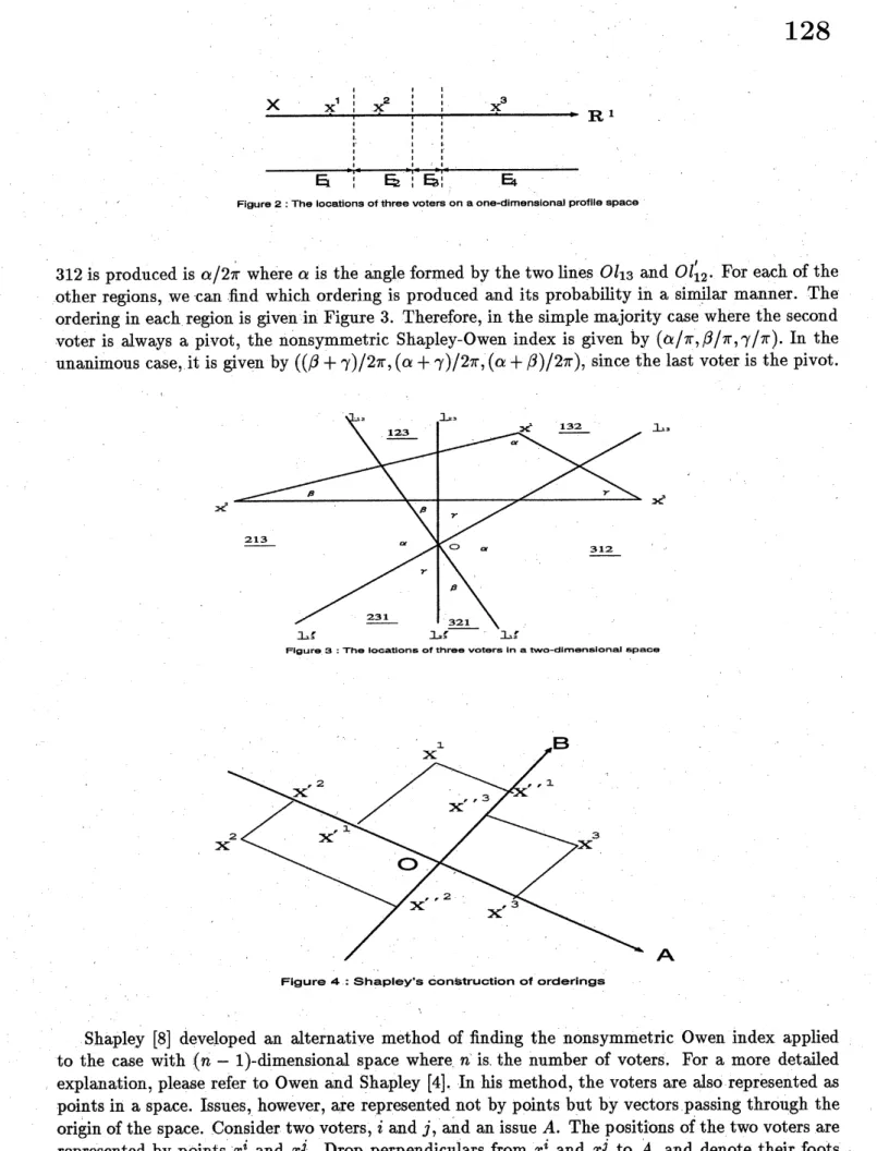
Owen [3] introduced an ideology profile space to considerthe nonsymmetry of voters. If there is only one ideological axis, for example, a left-right axis, then
the case of the three voters can be depicted in terms of aline as in Figure 2. For each$i=1,2,3,$ $x^{i}$
denotes the position ofvoter $i$
.
The midpoints of the line segments $x^{1}x^{2},x^{1}x^{3}$ and $x^{2}x^{3}$ serve as theborders which divide the line into four regions, $E_{1},$ $E_{2},$$E_{3}$ and $E_{4}$
.
For any bill in region $E_{1}$, voter 1is the closest, voter 2 is the next closest, and voter 3 is the most distant. Thus, the grand $\mathrm{c}\mathrm{o}A\mathrm{t}\mathrm{i}\mathrm{o}\mathrm{n}$
is formed in the order 123. Similarly in regions $E_{2},$$E_{3}$ and $E_{4}$, the orderings are 213, 231 and 321.,
respectively. It should be noted that regions $E_{1}$ and $E_{4}$ are unbounded intervals. This implies that
ifbills arise at random along the whole real line, orderings 123 and 321 would appear at an equal
probability of 0.5. In asimple majority case, voter 2 is pivotal in both orderings. Thus, voter 2 has
ffi of the power. In a unanimous case, voter 3 is pivotal in 123 and voter 1 is pivotal in 321. In this
case, voters 1 and 3 have equal power of 0.5 and voter 2 is powerless.
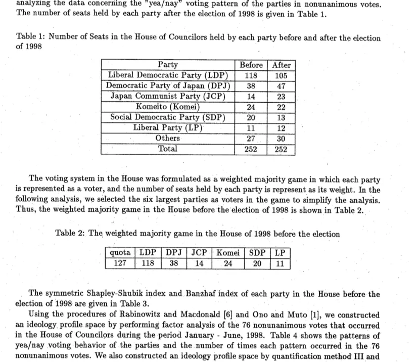
Figure 3 depicts the cas$e$ofthree vot$e\mathrm{r}\mathrm{s}$in a two-dimensionalspace. Each$x^{i}$ denotes the position
of voter $i$
.
Since there are three points, there arethree perpendicular bisectors which intersect the
midpoint of the lines which connect each pair of points. In Figure 3, the line $l_{ij}-l_{ij}’$ represents the
perpendicular bisector of$x^{i}$ and $x^{j},j=1,2,3,$
$i\neq j$
.
For instance, $\mathrm{b}\mathrm{i}$]$\mathrm{l}\mathrm{s}$ inthe sector formed by the
half-lines $Ol_{13}$ and $OI_{12}^{l}$ produce the ordering 312, since for any bin in this region, voter 3
is the
most enthusiastic supporter, voter 1 is the next enthusiastic, and voter 2 is the least enthusiastic.
$\frac{\mathrm{X}\mathrm{x}^{\tau}1||\mathrm{x}^{2}111\dagger l}{1|,111’ 1||111111}$ . $|11\mathrm{I}\mathrm{l}\mathrm{l}\mathrm{I}l111$ $\mathrm{x}^{3}$ $\mathrm{R}^{1}$ $\mathrm{B}$
$1\mathrm{t}$ $\mathrm{B}\mathrm{l}\mathrm{l}\mathrm{B}_{1}^{\mathrm{I}}$ $\mathrm{B}$
Figure2:The$\mathrm{I}\mathrm{o}\mathrm{c}\mathrm{a}2\mathrm{l}\mathrm{o}\mathrm{n}\mathrm{s}$ofthree votersona$\mathrm{o}\mathrm{n}\mathrm{e}-\mathrm{d}\dot{\mathrm{l}}\mathrm{m}\mathrm{e}\mathrm{n}\mathrm{s}\mathrm{i}\mathrm{o}\mathrm{n}\mathrm{a}\mathrm{I}$profllespace
312isproduced is $\alpha/2\pi$ where $\alpha$ is the angleformed by the two lines $Ol_{13}$ and $Ol_{12}’$
.
For each of theother regions, we can find which ordering is produced and its probability in a similar manner. The
orderingin each region is given in Figure 3. Therefore, in the simple majority case where the second
voter is always a pivot, the nonsymmetric Shapley-Owen index is given by $(\alpha/\pi,\beta/\pi,\gamma/\pi)$
.
In theunanimous case, it is given by $((\beta+\gamma)/2\pi, (\alpha+\gamma)/2\pi,$ $(\alpha+\beta)/2\pi)$, since the last voteris the pivot.
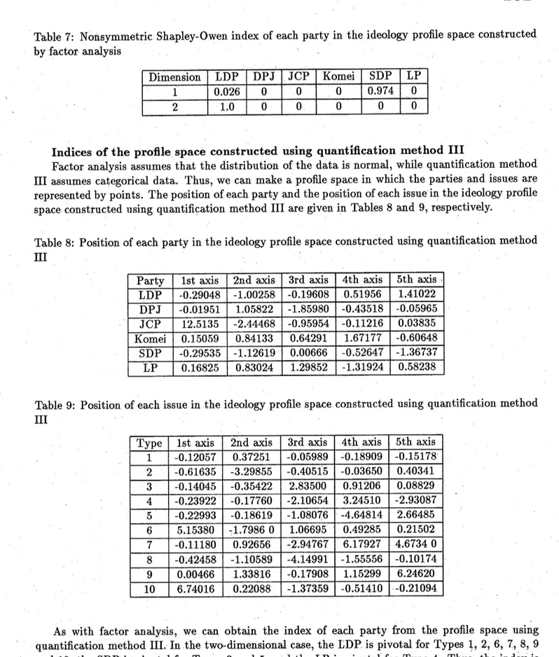
Figure 4 :ShapIey$\mathrm{s}\mathrm{c}\mathrm{o}\mathrm{n}\mathrm{B}\mathrm{t}\mathrm{r}\mathrm{u}\mathrm{c}\mathrm{t}\mathrm{i}\mathrm{o}\mathrm{n}$of orderings
Shapley [8] developed an alternative method of finding the nonsymmetric Owen index applied
to the case with $(n-1)$-dimensional space where $n$ is.the number of voters. For a
more
detailedexplanation, pleace refer to Owen and Shapley [4]. In his method, the voters are also represented as
pointsin a space. Issues, however,
are
representednot by points but by vectors passing through theoriginof the space. Consider two voters, $i$ and$j$, and an issue$A$
.
The $\mathrm{p}\mathrm{o}\mathrm{s}\mathrm{i}\mathrm{t}\mathrm{i}\cdot \mathrm{o}\mathrm{n}\mathrm{s}$ ofthe two votersare
represented by points $x^{i}$ and $x^{j}$
.
Drop perpendiculars from $x^{i}$ and $x^{j}$ to $A$,
and denote their footsby $x^{i}$’ and $x^{j}’$, respectively. In this model, voter $i$ prefers $A$
more
than$j$ does, or $i$ precedes$j$ withrespect to $A$, if $||Ox^{i}||’>||Ox^{j}||$
’
where $O$ is the origin of the space and $||Ox^{i}||$
’
or $||Ox^{j}||$’ is the
distance dong the arrow $A$ between $O$ and $x^{i}’$
,
or between $O$ and $x^{j}’$,
respectively. In FiguTe 4, forfor issue $B$ is 132. If
we
rotate thearrow
around theorigin assuming that issues ariseat random,
wefind for each ordering the sector in which it is produced. For each ordering the proportion of the
corresponding angle to $2\pi$ gives the probability at which the ordering appears. The nonsymmetric
indexis obtained byfinding a pivotal voterin an arbitrary position. The
same
indices are obtainedevenifthe origins are different. Thenonsymmetricindex produced by this method is often called the
Shapley-Owen index.
3
Application of the
nonsymmetric Shapley-Owen index to the
voting
behavior
of the Japanese
House
of
Councilors
in
January-June, 1998
Weevaluated the power of each party in the Japanese House of Councilors in 1998. In theelection of
1998, the LDP did not regain a majority of seats in the House. The LDP had held a majority until
the election of 1989. After the election of 1989, they lost the majority, and this produced movement
by many renewal parties such as the Liberal Party and the Democratic Party of Japan. Ono and
Muto [1] analyzed the power of each party in the House during the period 1989-1992. In this study,
we investigated the power of each party in the House during the period of January-June, 1998 by
analyzing the data concerning the ”
$\mathrm{y}\mathrm{e}\mathrm{a}/\mathrm{n}\mathrm{a}\mathrm{y}$” voting pattern of the parties in nonunanimous votes.
The number of seats held by each party after the election of 1998 is given in Table 1.
Table 1: Number of Seats in the House of Councilors held by each party before and after the election of1998
Thevoting systemin the Housewasformulated as a weighted majority game in which each$\mathrm{p}\mathrm{a}\mathrm{T}\mathrm{t}\mathrm{y}$
is representedas avoter, and the number of seats held by each party is representas its weight. In the
following analysis, we selected the six largest parties as voters in the game to simplify the analysis.
Thus, the weighted majoritygame in the IIouse before the election of 1998is shownin Table 2.
Table 2: The weighted majoritygame in the House of 1998 before the election
The symmetric Shapley-Shubikindex and Banzhaf index of each party in the
Hous.e.
before theelection of 1998
are
given in Table3.Using the procedures of Rabinowitz and Macdonald [6] and Ono and Muto [1], we constructed
an ideology proffie space by performing factor analysis ofthe 76 nonunanimous votes that occurred
in the House of Councilors during the period January- June, 1998. Table 4 shows the patterns of
$\mathrm{y}\mathrm{e}\mathrm{a}/\mathrm{n}\mathrm{a}\mathrm{y}$voting behavior of the parties and the number of times each pattern occurred in the 76
Table 3: Shapley-Shubikindex and Banzhafindex ofeachparty
Index LDP DPJ JCP Komei SDP LP
Shapley-Shubik $.835$ $.033$ $.033$ $.033$ $.033$ $.033$
Banzhaf $.968$ $.031$ $.031$ $.031$ $.031$ $.031$
evaluated the indices of this profile space.
Table
4:
Pattern of$\mathrm{y}\mathrm{e}\mathrm{s}/\mathrm{n}\mathrm{o}$ voting of the 6 parties in the 76 nonunanimous votes during January-June,1998 (Sangiin Kaigiroku [7])
Type LDP DPJ Komei SDP JCP LP Number
$1$ $\mathrm{Y}$ $\mathrm{Y}$ $\mathrm{Y}$ $\mathrm{Y}$ $\mathrm{N}$ $\mathrm{Y}$ $50$
$2$ $\mathrm{Y}$ $\mathrm{N}$ $\mathrm{N}$ $\mathrm{Y}$ $\mathrm{N}$ $\mathrm{N}$ $12$
$3$ $\mathrm{Y}$ $\mathrm{N}$ $\mathrm{Y}$ $\mathrm{Y}$ $\mathrm{N}$ $\mathrm{Y}$ $6$
$4$ $\mathrm{Y}$ $\mathrm{Y}$ $\mathrm{Y}$ $\mathrm{Y}$ $\mathrm{N}$ $\mathrm{N}$ $2$
$5$ $\mathrm{Y}$ $\mathrm{Y}$ $\mathrm{N}$ $\mathrm{Y}$ $\mathrm{N}$ $\mathrm{Y}$ $1$
$6$ $\mathrm{Y}$ $\mathrm{N}$ $\mathrm{Y}$ $\mathrm{Y}$ $\mathrm{Y}$ $\mathrm{Y}$ $1$
$7$ $\mathrm{Y}$ $\mathrm{Y}$ $\mathrm{Y}$ $\mathrm{N}$ $\mathrm{N}$ $\mathrm{N}$ $1$
$8$ $\mathrm{Y}$ $\mathrm{Y}$ $\mathrm{N}$ $\mathrm{Y}$ $\mathrm{N}$ $\mathrm{N}$ $1$
$9$ $\mathrm{Y}$ $\mathrm{Y}$ $\mathrm{Y}$ $\mathrm{N}$ $\mathrm{N}$ $\mathrm{Y}$ $1$
$10$ $\mathrm{N}$ $\mathrm{Y}$ $\mathrm{Y}$ $\mathrm{N}$ $\mathrm{Y}$ $\mathrm{Y}$ $1$
Indices of the profile space constructed using factor analysis
Factor analysis showed that the first main factor accounted for 41.011 percent of the variance in
tihe 76 votes, and that the second factor accounted for 34.354percent of the variance.
Table 5: Position of each party in the ideology profile space constructed using factor analysis
Party 1st factor 2nd factor 3rd factor 4th factor 5thfactor
LDP $0.58120$ $1.08979$ $-0.21761$ $0.52755$ $1.92172$ DPJ $0.24418$ $-1.04659$ $-1.71312$ $-0.27420$ $-0.04130$ JCP $-2.02265$ $0.26989$ $0.26500$ $0.03890$ $0.02193$ Komei $0.34389$ $-0.76896$ $0.76362$ $1.59576$ $-0.57231$ SDP $0.54723$ $1.21513$ $-0.05561$ $-0.54636$ $-1.44536$ LP $0.30615$ $-0.75921$ $1.11962$ $-1.34165$ $0.51532$
Table6: Direction of each type ofissue inthe ideologyprofile space constructed using factoranalysis
Therefore, the first two factors accounted for 75.365percent of the variance. Tables 5 and 6 show
the position of each party and the direction of each type of issue, respectively, in the profile space.
Figure 5 shows the two-dimensionalprofile space constructed using factor analysis.
Figure5:Two-dimensionalprofiIespaceconstructedbyfactoranalysis
Figure 5 shows that the observed issues
are
not uniformly distributed. The nonuniformity ofissuesis intrinsic to our study because bills are mainly submitted by acabinet, in which most of the
membersbelongtothegoverningparty. The nonsymmetric Shapley-Owen index
assumes
randomnessof the $\mathrm{b}\mathrm{i}\mathrm{U}\mathrm{s}$
.
The results of thefactor analysis do not meet this assumption. Therefore, we employed
the method of Ono and Muto [1] to calculate the nonsymmetricindex using only the data. Thus, the
obtained index shows only the power distribution during January-June, 1998, and does not predict
future votingbehavior. We need to find a pivotal party for each type ofissuein the two-dimensional
case. For all types of issues, the LDP is the pivot. For example, the order of type 5 is $\mathrm{S}\mathrm{D}\mathrm{P}arrow \mathrm{L}\mathrm{D}\mathrm{P}$
$arrow \mathrm{K}\mathrm{o}\mathrm{m}\mathrm{e}\mathrm{i}arrow \mathrm{L}\mathrm{P}arrow \mathrm{D}\mathrm{P}\mathrm{J}arrow \mathrm{J}\mathrm{C}\mathrm{P}$,
and the LDP is the pivot. Thus, the index for LDP is $76/76=1$
.
The indices of the other five parties are$0$
.
Thein.dices
forthe.one-dimensional
case are also noted inTable 7: Nonsymmetric Shapley-Owen index of each party in the ideology proffie space construct$e\mathrm{d}$
byfactor analysis
Indices ofthe profile space constructed using
quantification
method IIIFactor analysis assumes that the distribution of the data is normal, while quantification method
III assumes categorical data. Thus, we can make a proffie space in which the parties and issues
are
represented by points. Theposition of each party and the position of each issue in the ideology proffie
space constructed using quantification method III are given in Tables 8 and 9,respectively.
Table 8: Position of each party in the ideology profile space
constructed
using quantification methodIII
Party 1st axis 2nd axis 3rd axis 4th axis 5th axis
LDP $-0.29048$ $-1.00258$ $-0.19608$ $0.51956$ $1.41022$ DPJ $-0.01951$ $1.05822$ $-1.85980$ $-0.43518$ $-0.05965$ JCP $12.5135$ $-2.44468$ $-0.95954$ $-0.11216$ $0.03835$ Komei $0.15059$ $0.84133$ $0.64291$ $1.67177$ $-0.60648$ SDP $-0.29535$ $-1.12619$ $0.00666$ $-0.52647$ $-1.36737$ LP $0.16825$ $0.83024$ $1.29852$ $-1.31924$ $0.58238$
Table 9: Position of each issue in the ideology profile space constructed using quantification method
III
Typ$e$ 1st axis 2nd axis 3rd axis 4th axis 5th axis
$1$ $-0.12057$ $0.37251$ $-0.05989$ $-0.18909$ $-0.15178$ $2$ $-0.61635$ $-3.29855$ $-0.40515$ $-0.03650$ $0.40341$ $3$ $-0.14045$ $-0.35422$ $2.83500$ $0.91206$ $0.08829$ $4$ $-0.23922$ $-0.17760$ $-2.10654$ $3.24510$ $-2.93087$ $5$ $-0.22993$ $-0.18619$ $-1.08076$ $-4.64814$ $2.66485$ $6$ $5.15380$ $-1.79860$ $1.06695$ $0.49285$ $0.21502$ $7$ $-0.11180$ $0.92656$ $-2.94767$ $6.17927$ $4.67340$ $8$ $-0.42458$ $-1.10589$ $-4.14991$ $-1.55556$ $-0.10174$ $9$ $0.00466$ $1.33816$ $-0.17908$ $1.15299$ $6.24620$ $10$ $6.74016$ $0.22088$ $-1.37359$ $-0.51410$ $-0.21094$ .
As with factor analysis, we can obtain the index of each party from the proffie space using
quantification method III. In the two-dimensiondcase, the LDP is pivotal for Types 1, 2, 6, 7, 8, 9
and 10; the SDP is pivotal for Types 3 and 5; and the LP is pivotal for Type 4. Thus, the indexis
$(50+12+1+1+1+1+1)/76=0.882$ for
the
LDP; $(6+2+1)/76=0.118$forthe SDP. Table 10 givesthe non-symmetric Shapley-Owen index of each party for theone-dimensional and two-dimensional
cases.
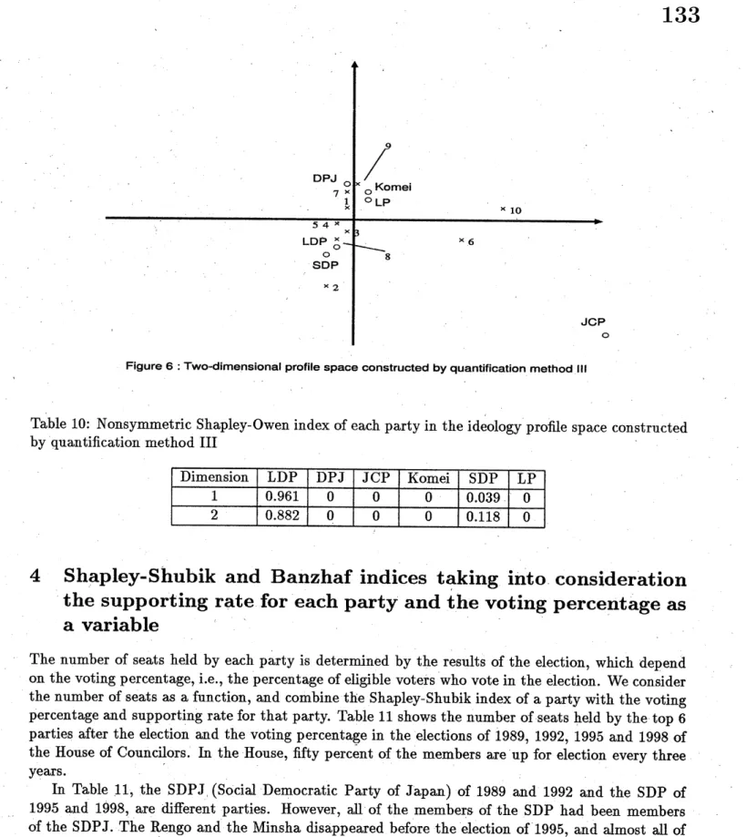
Theindices obtained using quantification method III are more realistic than those obtainedusingfactor analysis. The index values of eachparty show thatthe LDP has alargeamount ofpower,
Figure6:Two-dimensional profilespaceconstructedby quantification method III
Table 10: Nonsymmetric Shapley-Owen index of each party in the$\mathrm{i}\mathrm{d}\dot{\mathrm{e}}\mathrm{o}\mathrm{l}\mathrm{o}\mathrm{g}\mathrm{y}$
profilespace constructed
by quantification method III
Dimension LDP DPJ JCP Komei SDP LP
$1$ $0.961$ $0$ $0$ $0$ $0.039$ $0$ $2$ $0.882$ $0$ $0$ $0$ $0.118$ $0$
4
Shapley-Shubik and Banzhaf
indices taking
into consideration
the
supporting rate
for each
party
and
the
voting.
percentage
as
a
variable
Thenumber of seats held by each party is determined by the results of the election, which depend
on the voting percentage, i.e., the percentage of eligible voters who vote in the election. We consider
the number ofseats as a function, and combine the Shapley-Shubik index of a party with the voting
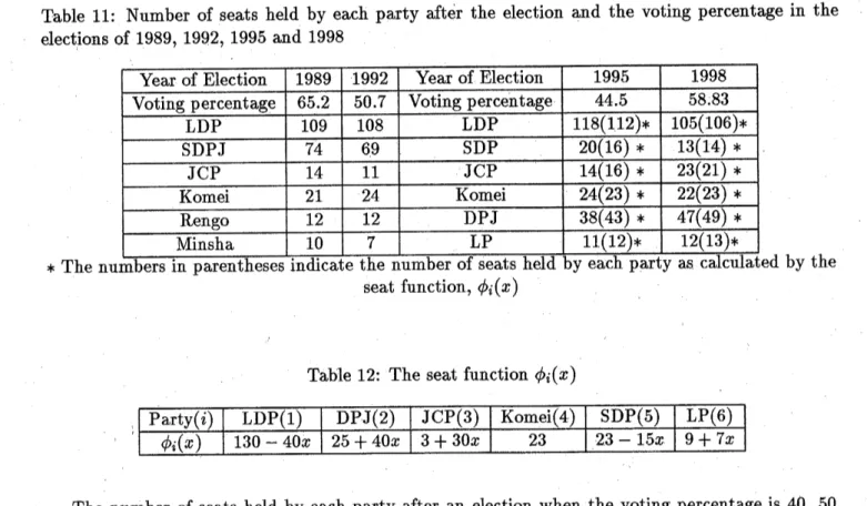
percentage and supporting rate for that party. Table 11 shows the number of seats held by the top 6
parties after the election and the voting
percenta.g
$\mathrm{e}$ in the elections of 1989, 1992, 1995 and 1998 ofthe House of Councilors. In the House, fifty percent ofthe members are up for election every three
years.
In Table 11, the SDPJ (Social Democratic Party of Japan) of 1989 and 1992 and the SDP of
1995 and 1998, are different parties. However, ffi of the members of the SDP had been members
of the SDPJ. The Rengo and the Minsha disappeared before the election of 1995, and almost all of
the members ofthese two parties joined the
new
DPJ party. By regression analysis of the numberof seats, where the independent variable is the number of seats held by a particular party after an
election and the dependent variable is the voting percentage in the 4 elections, only the Komei had
ahigh $R^{2}=0.921$
.
The$R^{2}$ ofthe other parties wasat most 0.559, whichindicates that the number
of seats held by of each party cannot be estimated by the voting percentage. Thus,
we
arbitrarilymade the seat function, $\phi_{i}(x),i=1,$$\cdots,6$ of the number of seats held by party after an $i$ as folows,
where$x$ is the voting percentagein theelection of members of the House. It is said in Japan that at
higher voting percentages, the number of seats held by the LDP after
an
election decreases, and thenumber of seats held by the DPJ increases. The numbers in parentheses in Table 11 correspond to
Table 11: Number of seats held by each party after the election and the voting percentage in the
$\mathrm{e}\mathrm{l}\mathrm{e}\mathrm{e}^{\backslash }r\mathrm{t}_{}\mathrm{i}\mathrm{o}\mathrm{n}\mathrm{s}$ of 1989. 1992. 1995 and 1998
Table 12: The seat function $\phi_{i}(x)$
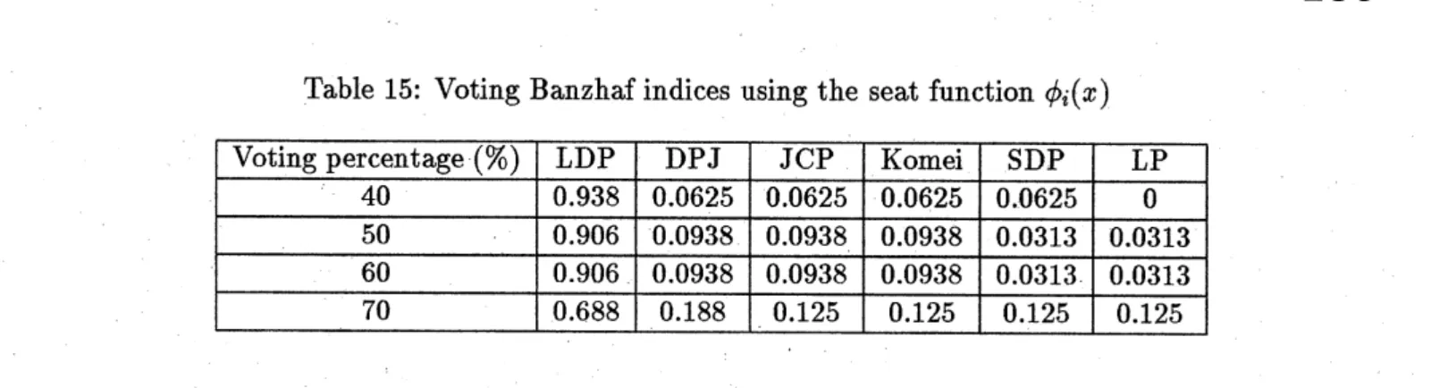
The number of seats held by each party after an election when the voting percentage is 40, 50,
60, or 70 percent, as calculated by the seat function $\phi$, is given in Table 13. Tables 14 and 15 give
the Voting-Shapley-Shubikindex and the Voting-Banzhafindex, respectively, of each party when the
voting percentage varies between 40 and 70 percent. The indices suggest that as the voting percentage
increases, the LDP loses power but wouldstin have the largest amount of power among the parties.
Table 13: Number of seats held by each party after the election according to the seat function $\phi_{i}(x)$
Voting percentage (%) LDP DPJ JCP Komei SDP LP
$40$ $114$ $41$ $15$ $23$ $17$ $12$
$50$ $110$ $45$ $18$ $23$ $16$ $13$
$60$ $106$ $49$ $21$ $23$ $14$ $13$
$70$ $102$ $53$ $24$ $23$ $12$ $14$
Table 14: Voting Shapley-Shubik indices usingthe seat function $\phi_{i}(x)$
Voting percentage (%) LDP DPJ JCP Komei SDP LP
$40$ $0.800$ $0.0500$ $0.0500$ $0.0500$ $0.0500$ $0$ $50$ $0.767$ $0.0667$ $0.0667$ $0.0667$ $0.0167$ $0.0167$ $60$ $0.767$ $0.0667$ $0.0667$ $0.0667$ $0.0167$ $0.0167$ $70$ $0.533$ $0.133$ $0.0833$ $0.0833$ $0.0833$ $0.0833$
Table 15: VotingBanzhaf indices using the seat function $\phi_{i}(x)$
Voting percentage (%) LDP DPJ JCP Komei SDP LP
$40$ $0.938$ $0.0625$ $0.0625$ $0.0625$ $0.0625$ $0$ $50$ $0.906$ $0.0938$ $0.0938$ $0.0938$ $0.0313$ $0.0313$ $60$ $0.906$ $0.0938$ $0.0938$ $0.0938$ $0.0313$ $0.0313$ $70$ $0.688$ $0.188$ $0.125$ $0.125$ $0.125$ $0.125$
As the next step,weconsidered both thevotingpercentage and thesupportingrate for each party,
i.e., the percentage of eligible voters who support a particular party, and made the seat function
dependent on these two factors. The supporting rates for each party in 1998 are given in Graph 1.
There are, however, voters who support a party but don’t vote. We assume that they comprise 20.3
percent of ffi eligible voters. We also assume that 40 percent ofall voters support a party and vote
for that party. This implies that the lowest voting percentage is 40 percent and the highest is 79.7
percent(see Graph 2). TheJCP and Komei have$\mathrm{w}\mathrm{e}\mathrm{U}$-organized,strong systems ofvoting
amongtheir
members. Therefore, 90 percent of the supporters of the JCP and Komeiareassumed to vote. Political
independents comprise 39.7 percent ofall voters. Their voting behavior is important for ffi parties.
We assumed that the political independents voted for the respective parties at the rates indicated in
Graph 3; these data were obtained from a public opinion $\mathrm{p}\mathrm{o}\mathrm{U}$ conducted by Kyoudoutuusinsya on
July 15, 1998.
Graph1 Supponngratesforeachpanyin 1998
uvope$e$.vmng$\mathrm{r}.\mathrm{a}\mathrm{I}\mathrm{e}\mathrm{s}\mathrm{I}\Pi$an$\mathrm{e}\mathrm{l}\mathrm{e}-$ $\mathrm{c}*\mathrm{r}\mathrm{a}\mathrm{p}\mathrm{n}\mathrm{s}$: YoIlng$\mathrm{o}\mathrm{e}\mathrm{n}\mathrm{a}\mathrm{v}l\mathrm{o}\mathrm{r}$or$\mathrm{p}\mathrm{o}\mathrm{I}\mathrm{l}\mathrm{I}\mathrm{t}\mathrm{c}\mathrm{a}\mathrm{l}$
independentsIn$1_{\vee}^{\mathrm{C}}$
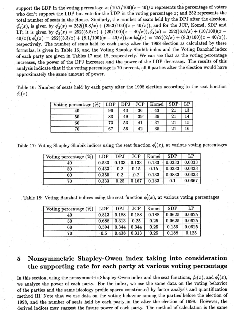
Therefore, when the voting percentage is $x$ and the supporting rate is given by the graphs, the
numberof seats,$\phi_{1}^{J}(x)$, held bythe LDP after the election of 1998can be determinedby the equation,
support the LDP in the voting percentage$x;(10.7/100)(x-40)/x$ representsthepercentageof voters
whodon’t support the LDP but vote for the LDP in the votingpercentage$x$; and 252 represents the
totalnumber of seats in theHouse. Similarly, the number ofseats heldbythe DPJ after the election,
$\phi_{2}’(x)$, is given by $\phi_{2}’(x)=252((6.8/x)+(29.3/100)(x-40/x))$, and for the JCP, Komei, SDP and
$\mathrm{L}\mathrm{P}$, it is given by $\phi_{3}’(x)=252((5.8/x)+(20/100)(x-40/x)),\phi_{4}’(x)--252((6.8/x)+(10/100)(x-$
$40/x)),\phi_{5}’(x)=252((3.3/x)+(8.1/100)(x-40/x)),\mathrm{a}\mathrm{n}\mathrm{d}\phi_{6}’(x)=252((2/x)+(8.3/100)(x-40/x))$
,
respectively. The number of seats held by each party after the 1998 election as calculated by these
formulas, is given in Table 16, and the Voting Shapley-Shubik ind$e\mathrm{x}$ and the Voting Banzhafindex
of each party are given in Tables 17 and 18, respectively. We can see that as the voting percentage
increases, the power of the DPJ increases and the power of the LDP decreases. The results of this
analysisindicate that if the voting percentage is 70 percent, alll 6 parties after the election would have
approximately the same amount of power.
.
Table 16: Number of seats held by each party after the 1998 election according to the seat function
$\phi_{i}^{J}(x)$
Voting percentage (%) LDP DPJ JCP Komei SDP LP
$40$ $96$ $43$ $36$ $43$ $21$ $13$
$50$ $83$ $49$ $39$ $39$ $21$ $14$
$60$ $73$ $53$ $41$ $37$ $21$ $15$
$70$ $67$ $56$ $42$ $35$ $21$ $16$
Table 17: Voting Shapley-Shubik indices using the seat function $\phi_{i}’(x)$, at various voting percentages
Voting percentage (%) LDP DPJ JCP Komei SDP LP
$40$ $0.533$ $0.133$ $0.133$ $0.133$ $0.0333$ $0.0333$
$50$ $0.433$ $0.2$ $0.15$ $0.15$ $0.0333$ $0.0333$
$60$ $0.350$ $0.2$ $0.2$ $0.133$ $0.0833$ $0.0333$
$70$ $0.333$ $0.25$ $0.167$ $0.133$ $0.1$ $0.0667$
Table 18: Voting Banzhaf indices using the seat function $\phi_{i}’(x)$, at various voting percentages
Voting percentage (%) LDP DPJ JCP Komei SDP LP
$40$ $0.813$ $0.188$ $0.188$ $0.188$ $0.0625$ $0.0625$ $50$ $0.688$ $0.313$ $0.25$ $0.25$ $0.0625$ $0.0625$
$60$ $0.594$ $0.344$ $0.344$ $0.25$ $0.156$ $0.0625$
$70$ $0.5$ $0.438$ $0.313$ $0.25$ $0.188$ $0.125$
5
Nonsymmetric
Shapley-Owen
index taking
into
consideration
the
supporting
rate
for
each party at
various voting
percentage
In this section,using the nonsymmetric Shapley-Owen index and the seat functions, $\phi_{i}(x)$, and $\phi_{i}’(x)$,
we
analyze the power of each party. For the index,we use
thesame
dataon
the voting behaviorof the parties and the
same
ideology profile spacesconstructed
by factor analysis and quantificationmethod III. Note that we use data on the voting behavior among the parties before the election of
1998, and the number of seats held by each party in the after the election of 1998. However, the
derived indices may suggest the future power of each party. The method ofcalculation is the same
as
that in Section 3. Thus, we present only the results of the two-dimensional casein Tables 19-22.power. This may be the
reason
$\dot{\mathrm{t}}$hat since January, 1999, the LDP has been exploring the possibility
ofmaking a$\mathrm{c}\mathrm{o}\mathrm{A}\overline{\mathrm{t}}\mathrm{i}\mathrm{o}\mathrm{n}$ cabinet with the Komei.
Table 19: Nonsymmetric Shapley-Owenindex of each$\mathrm{p}\mathrm{a}\mathrm{r}\dot{\mathrm{t}}\mathrm{y}$
in the profile $\mathrm{s}.\mathrm{p}$ace
c.onstructed
byfactoranalysis and the function $\phi_{i}(x),\mathrm{a}\mathrm{t}$ various votingpercentages
Table 20: Nonsymmetric Shapley-Owen index of each party in the profile space constructed by
quantification method III and the function $\phi_{i}(x)$, at various voting percentages
Table 21: Nonsymmetric Shapley-Owen index ofeachpartyin the profile space constructed by factor
analysis and thefunction $\phi_{i}’(x)$, at various voting percentages
Table 22: Nonsymmetric Shapley-Owen index of each party in the profile space constructed by
quantification method III and the function $\phi_{i}’(x)$, at various voting percentages
6
Conclusion
In conclusion, we mention that when the voting percentage varies and the supporting rates for each
party differ, analysis of power indices may be helpful in estimating the powerof each
par.ty
aft.er
anelection,ifwe can make a reliable seat function.
Acknowledgments
REFERENCES
1. Ono, R. and Muto, S., Party Power in the House
of
Councilors in Japan: An Applicationof
the Nonsymmetric Shapley-Owen Index, Journal of the Operations Research Society of Japan,
40 (1997), 21-33.
2. Owen, G., Political Games, Naval Research Logistics Quarterly, 18 (1971), 345-355.
3. Owen, G., Game Theory, Third edition, Academic Press, 1995.
4. Owen, G. and Shapley, L. S., OptimalLocation
of
Candidates in Ideological Space,InternationalJournal of Game Theory, 18 (1989), 339-356.
5. Imidas (in Japanese), (1998) Syueisya.
6. Rabinowitz, G. and Macdonald, S. E., The Power
of
the States in $U.S$.
PresidentialElections,American Political Science Review, 80 (1986), 65-87.
7. Sangiin Kaigiroku (in Japanese), (1998). Okurasyo-Insatukyoku.
8. Shapley, L. S., A Comparison