Aharonov-Bohm Effect in Scattering by a Chain of Point-like Magnetic Fields (Spectral and Scattering Theory and Related Topics)

Aharonov-Bohm

Effect

in

Scattering

by

a

Chain of Point-like

Magnetic

Fields

Hiroshi

T.

Ito

(

伊藤 宏

)

and Hideo Tamura

(

田村 英男

)

Department ofComputer Science, Ehime University

Matsuyama 790-8577, Japan

and

DepartmentofMathematics, Okayama University

Okayama 700-8530, Japan Abstract 量子力学に従う粒子が直接磁場に触れていなくても, ベクトル・ポ テンシャルからの影響をうけ, 離れた場所の磁場を感じる現象は Aharonov-Bohm 効果として知られている ([3]). 複数個の

2

次元 $\delta$ 型磁場 $\underline{(}\mathrm{m}\mathrm{a}\mathrm{g}\mathrm{n}\mathrm{e}\mathrm{t}\mathrm{i}\mathrm{c}$ vortex[8] $)$ によ る散乱を考え, 磁場の中心を大きく離したときの散乱振幅の漸近公式を導く

.

各磁 場による散乱がポテンシャル (長距離型摂動となる) を通していかなる相互作用を 及ぼしあうかを解析するのが目的である. 結果には入射方向・散乱方向や各磁場の フラックスのみならず磁場のお互いの位置関係が反映する. 特に, 入射方向または散 乱方向に沿って複数の $\delta$ 型磁場が並んでいる場合にはそれ以外の場合とは異なった 興味深い結果が得られた. 証明については [6] を参照してください.

Introduction and Results

Westudy the magnetic scattering by several point-likefields at large separation

in two dimensions. The aim is to derivethe asymptotic formula for scattering

am-plitudes

as

thedistances between centers of fields go to infinity. Even ifamagnetic

fieldis compactly supported, the corresponding vector potential doesnotnecessarily

falloffrapidly, and in general, it has the long-range propertyat infinity. We discuss

from amathematical point of view how the scattering by separate fields interacts

with

one

another through long-range magnetic potentials. Aspecial emphasis is

placed

on

the

case

ofscatteringbyfields with centers

on an even

Hoe. Theobtained

resultdepends

on

fluxesof fieldsand

on

ratiosof distancesbetween adjacentcenters.

It is known

as

the Aharonov-Bohm effect ([3]) that magnetic potential has adirect

significance to the motion ofquantum particles. An extensive list of physical

liter-atures

on

theAharonov-Bohmscattering

can

be found in the book [2]. We refer to

therecent article [8] for the Aharonov-Bohm effect in manypoint-like fields, where

the term magnetic vortexis used for point-like magnetic field.

Throughout thewhole exposition,

we

work in the twodimensional space$R^{2}$with

数理解析研究所講究録 1255 巻 2002 年 143-151

generic point

x

$=(x_{1},x_{2})$

.

Wewrite

$H(A)=(-|. \nabla-A)^{2}=\sum_{j=1}^{2}(-\dot{l}\partial_{j}-a_{j})^{2}$, $\partial_{\dot{f}}=\partial/\ _{j}$,

$=(a_{1}(x),a_{2}(x))$

:

$b=\nabla \mathrm{x}A=\mathrm{d}a_{2}-\ a_{1}$

and the quantity $\alpha=(2\pi)^{-1}\int b(x)dx$ is calld the total flux of field $b$

,

where the

integration with

no

domain attached is taken

over

the whole space. We often

use

this abbreviation.

We

first

consider the

case

of

asingle point-like

field.

The Hamiltonian

with

such afield is regarded

as one

of solvable models and the explicitrepresentationfor

scattering amplitude has been already obtained by [1, 2, 9]. Let $2\pi\alpha\delta(x)$ be the

magnetic field

with

flux $\alpha$ and center at the origin. Then the magnetic potential

$A_{\alpha}(x)$ associated with the fieldis given by

$A_{a}(x)=\alpha$(-&log$|x|$

,

a

$\log|x|$) $=\alpha(-x_{2}/|x|^{2},x_{1}/|x|^{2})$

.

(1)

In fact,

we can

easily

see

that

$\nabla \mathrm{x}A_{a}=\alpha$$\mathrm{A}\log|x|=2\pi\alpha\delta(x)$

.

Weshould note that $A_{\alpha}(x)$ does not $\mathrm{f}\mathrm{a}\mathbb{I}$ offrapidly at infinity andit has the

long-rangeproperty. We write$H_{\alpha}=H(A_{a})$

.

Thepotential$A_{\alpha}(x)$ has strongsingularity

at theorigin,

so

that $H_{\alpha}$ is not necessarily essentialy self-adjoint in$C_{0}^{\infty}(R^{2}\backslash \{0\})$

$([1,4])$

.

We have toimpose

some

boundaryconditions at theoriginto define $H_{\alpha}$

as

aself-adjoint extension in $L^{2}=L^{2}(R^{2})$

.

We denote by the

same

notation $H_{\alpha}$ the

operator with domain

$D(H_{\alpha})=\{u\in L^{2} : H(A_{\alpha})u\in L^{2}, |x|arrow 01\dot{\mathrm{m}}|u(x)|<\infty\}$,

where $\mathrm{H}\{\mathrm{A}\mathrm{c}\mathrm{l}$)$\mathrm{u}$ is understood in

$\alpha$ (distribution sense). Then $H_{\alpha}$ is known to be

self-adjoint in$L^{2}$ and this operator is calld the Aharonov-Bohm Hamiltonian. If,

in particular, $\alpha\not\in Z$ is not

an

integer, $u\in D(H_{\alpha})$ is convergent to

zero as

$|x|arrow \mathrm{O}$

.

As

statedabove,theamplitude$f_{\alpha}(\omegaarrow\tilde{\omega};E)$for the

scattering&0m

initialdirection

$\omega$ $\in S^{1}$ to final

one

$\tilde{\omega}$ at energy $E>0$ has been already calculated. If

we

identify

thecoordinates

over

theunit circle $S^{1}$ with the azimuth angles&0m the positive

$x_{1}$

axis, then$f_{\alpha}(\omegaarrow\tilde{\omega};E)$ is explicitly represented

as

$f_{\alpha}=c(E)((\mathrm{c}\mathrm{o}\mathrm{e}\alpha\pi-1)\delta(\tilde{\omega}-\omega)-(:/\pi)\sin\alpha\pi e^{:[\alpha](\tilde{\omega}-\omega)}F_{0}(\tilde{\omega}-\omega))$ (2)

with$c(E)=(2\pi/i\sqrt{E})^{1/2}$, where theGaussnotation$[\alpha]$denotesthe maximal integer

not exceeding $\alpha$, and $F_{0}(\theta)$ is defined by $F_{0}=\mathrm{v}.\mathrm{p}.e^{\theta}\dot{.}/(e^{\theta}\dot{.}-1)$

.

We

move

tothe scattering by point-likefieldsupported

on

$N$points$d_{j}\in R^{2},1\leq$ $j\leq N$

.

We makelargethedistance $|d_{jk}|=|d_{k}-d_{j}|$ betweencenters$d_{j}$ and$d_{k}$ under

the assumption that

the direction $\hat{d_{jk}}=d_{jk}/|d_{jk}|$ remains fixed (3)

for aU pairs $(j, k)$ with$j\neq k$

,

$1\leq j$

,

$k\leq N$

.

We further

assume

that

$\max|d_{jk}|\leq c\dot{\mathrm{m}}\mathrm{n}|d_{jk}|$ (4)

for

some

$c>1$

.

Thesetwoassumptions

on

the locationof centers

are

alwaysassumed

to be fulfilled. By translation,

we

may

assume

$d_{1}$ to remain fixed,

so

that all the

centers

are

in adisk $\{|x|<cd\}$ with another $c>1$, where $d= \min|d_{jk}|$

.

We write

$H_{d}=H(A_{d})$, $A_{d}(x)= \sum_{j=1}^{N}A_{j}(x)=\sum_{j=1}^{N}A_{\alpha_{\mathrm{j}}}(x-dj)$, (5)

for the Schr\"odinger operator with field $\Sigma_{j=1}^{N}2\pi\alpha_{j}\delta(x-d_{j})$, where $A_{\alpha}(x)$ is defined

by (1). According to the results in [5], $H_{d}$ becomes aself-adjoint operator with

domain

$D(H_{d})=\{u\in L^{2} : H(A_{d})u\in L^{2}, |xd\varliminf_{j}|arrow 0|u(x)|<\infty, 1\leq j\leq N\}$

.

We alsoknowfrom [5] that the

wave

operators

$W_{\pm}(H_{d}, H_{0})=s- \lim_{tarrow\pm\infty}\exp(itH_{d})\exp(-itH_{0})$

exist and

are

asymptotically complete, where$H_{0}=-\Delta$ isthefree Hamiltonian. We

denote by $f_{d}(\omegaarrow\tilde{\omega};E)$ the scattering amplitude of pair $(H_{d}, H_{0})$

.

The aim is to

analyzethe asymptotic behavior

as

$darrow\infty$ of$f_{d}(\omegaarrow\tilde{\omega};E)$

.

We fix the notation to state the obtained results. We denote by $\gamma(\hat{x};\omega),\hat{x}=$

$x/|x|$, the azimuth anglefromdirection$\omega\in S^{1}$

.

Let _{$A_{j}(x)$}, _{$1\leq j\leq N$}, be

as

in (5)

and set

$H_{j}=H(A_{j})$, $1\leq j\leq N$

.

(6)

The operator $H_{j}$ admits aself-adjoint realization under the boundary condition

$\lim|x-d_{\dot{f}}|arrow 0|u(x)|<\infty$ at center$x=d_{j}$ and the scattering amplitudeofpair$(H_{j}, H_{0})$

is given by

$f_{i}(\omegaarrow\tilde{\omega};E)=\exp(-i\sqrt{E}d_{j}\cdot(\tilde{\omega}-\omega))f_{\alpha_{\mathrm{j}}}(\omegaarrow\tilde{\omega};E)$ ,

where $f_{\alpha}$ is defined by (2). The first main theorem is formulated

as

folows.

Theorem 1Let the notation be

as

above. Assume (3) and (4).

_If

$\omega$ $\neq\hat{d}_{jk}$ and

$\tilde{\omega}\neq\hat{d}_{jk}$

for

allpairs $(j,k)$ wiih$j\neq k$, $1\leq j$, $k\leq N$, and$\omega$ $\neq\tilde{\omega}$, then$f_{d}(\omegaarrow\tilde{\omega};E)$

obeys

$f_{d}( \omegaarrow\tilde{\omega};E)=\sum_{\mathrm{j}=1}^{N}\exp(i(\tau_{j}-\tilde{\tau}_{j}))f_{j}(\omegaarrow\tilde{\omega};E)+o(1)$

,

$darrow\infty$

,

there$\tau_{j}=\Sigma^{N}\succ_{-1,k\neq j}\alpha_{k}\gamma(\hat{d}_{kj};\omega)$ and$\tilde{\tau}_{\mathrm{j}}=\Sigma_{k=1,k\neq j}^{N}\alpha_{k}\gamma(\hat{d}_{kj};-\tilde{\omega})$

.

We

can

find

the Aharonov-Bohm effect in the theorem above.

As

is

seen

from

the asymptoticformula, the scattering by

field

$2\pi\alpha_{j}\delta(x-d_{j})$ is

influenced

by other

fields through the coefficient $\exp(|.\tau_{\dot{f}})$, although the centers of fields

are

far away

&0m

one

another. This

means

that vector potentials have adirect significance to

quantum particles moving in magneticfields. The magnetic effect is

more

strongly

reflected in the

case

when $\omega$ $=\hat{d}_{\dot{g}k}$

or

$\tilde{\omega}=\hat{d}_{jk}$

.

We add the

new

notation. We

interpret $\exp(i\alpha\gamma(\omega;\omega))$

as

$\exp(i\alpha\gamma(\omega;\omega)):=(1+\infty(:2\alpha\pi))/2=\mathrm{c}\mathrm{o}\mathrm{e}\alpha\pi\exp(\dot{l}\alpha\pi)$

.

Then the

same

asymptotic formula

as

in Theorem 1can be shown to remain true

even

for$\omega$ $=\hat{d}_{kj}$

or

$\tilde{\omega}=\hat{d}_{kj}$ under the assumption

that

there is

no

other center

on

$l_{jk}$ for $\mathrm{a}\mathbb{I}$pairs $(j, k)$

,

(7)

where$l_{\mathrm{j}k}$ isthe joiningthetwocenters$d_{\dot{f}}$ and$d_{k}$

.

We do not intend to prove this

result here. We have studied the

case

$N=2$ in [5]. If $N=2$

,

(7) is automatically

satisfied. For example,

we

have obtained that the $\ovalbox{\tt\small REJECT} \mathrm{d}$ scattering amplitude

obey

$f_{d}(\omegaarrow-\omega;E)=f_{1}(\omegaarrow-\omega;E)+(\mathrm{c}\mathrm{o}\mathrm{e}\alpha_{1}\pi)^{2}f_{2}(\omegaarrow-\omega;E)+o(1)$ (8)

for $\omega=\hat{d}_{12}$

.

Our

emphasis is placed

on

the

case

without (7). As atypicalcase,

we

study the

scattering by point-like fields withcenters

on an even

line. For brevity,

we

confine

ourselves to the simple

case

$N=3$

.

The argument extends to the general

case

$N\geq 4$

.

What is interesting is that the asymptotic formula depends not only on

fluxes of fields but also

on

ratios of distances betweenadjacent centers. We

assume

that three centers

are

along the direction $\omega_{1}=(1,0)$ in the order of$d_{1}$, $d_{2}$ and$d_{3}$

.

We further

assume

that

the ratio $|d_{23}|/|d_{12}|=\delta_{0}$ remains fixed (9)

for

some

$\delta_{0}>0$

.

This assumption

can

be weakened

as

$\mathrm{h}.\mathrm{m}_{darrow\infty}|d_{\mathfrak{B}}|/|d_{12}|=\delta_{0}$

.

We

define $\theta_{\pm}\pi$ as

$\theta_{\pm}\pi=$ angle between two vectors $(0, \pm 1)$ and $(1, -\delta_{0}^{1/2})$

.

(10)

It is obviousthat$\theta_{+}+\theta_{-}=1$ and $0<\theta_{-}<\theta_{+}<1$

.

If,for example, three centers

are

at

even

intervals, then$\delta_{0}=1$,

so

that $\theta_{\pm}$

are

determined

as

$\theta_{+}=3/4$and$\theta_{-}=1/4$

.

We are now in aposition to state the second main theorem.

Theorem 2Let the notation be as above. Assume that (9) $i_{\mathit{8}}$

satisfied. If

$\tilde{\omega}\neq\pm\omega_{1}$

for

the incident direction$\omega_{1}=(1,0)$, then $f_{d}=f_{d}(\omega_{1}arrow\tilde{\omega};E)$ behaves like

$f_{d}=e^{\alpha_{2}(\pi-\gamma(-\omega_{1j}-\tilde{\omega}))}.\cdot e^{\dot{l}a_{\theta}(\pi-\gamma(-\omega_{1j}-\tilde{\omega}))}f_{1}$

$+$ $(\cos\alpha_{1}\pi)e^{\alpha_{1}(\pi-\gamma(-I\tilde{d}))}.\cdot e^{\dot{l}\alpha_{3}(\pi-\gamma(-\tilde{\omega}))}-\omega_{1j}f_{2}\omega_{1j}$

$+$ $(\theta_{+}\cos(\alpha_{1}+\alpha_{2})\pi+\theta_{-}\cos(\alpha_{1}-\alpha_{2})\pi)e^{\alpha_{1}(\pi-\gamma(\omega_{1};-\tilde{\omega}))}.\cdot e^{\alpha_{2}(\pi-\gamma(\{d_{1;-\tilde{\omega}))}}.\cdot f_{3}+o(1)$

as

$darrow\infty$

,

where $f_{j}=f_{j}(\omega_{1}arrow\tilde{\omega};E)$

for

$1\leq j\leq 3$

.

Moreover the backward

scattering amplitude $f_{d}(\omega_{1}arrow-\omega_{1};E)$ obeys

$f_{d}=f1+(\cos\alpha_{1}\pi)^{2}f_{2}+(\theta_{+}\cos(\alpha_{1}+\alpha_{2})\pi+\theta_{-}\cos(\alpha_{1}-\alpha_{2})\pi)^{2}f_{3}+o(1)$

with $f_{j}=f_{j}(\omega_{1}arrow-\omega_{1}; E)$

.

We make several comments

on

the two theorems above.

Remark 1The quantity $|f_{d}(\omega_{1}arrow\tilde{\omega};E)|^{2}$ is

called

the differential

cross

section.

We figure the approximate values of

cross

sections obtained from the asymptotic

formula

on

the right side in the appendix and

we see

how the pattern ofinterferences

changes with three flux parameters $\alpha_{1}$, $\alpha_{2}$ and $\alpha_{3}$

.

Remark 2The idea in the proofofTheorem 2, in principle, enables

us

to prove

Theorem 1without assuming that $\omega\neq\hat{d}_{kj}$ and $\tilde{\omega}\neq\hat{d}_{kj}$

.

For example, it is pos

sible to extend Theorem 2to the

case

ofscattering by several chains of point-lice

fields. However the formula takes arather complicated form and

we

donot have yet

obtained aunified form of representation.

Remark 3If

we

make achangeofvariables$xarrow dy$

,

then Theorems 1and2canbe

easily

seen

to yield the asymptotic behavior at high energy ofscattering amplitudes

when the distances between centers offields remain fixed.

We write $R(z;H)=(H-z)^{-}$” _: $L^{2}arrow L^{2}$

,

${\rm Im} z\neq 0$

,

for the resolvent of

self-adjoint operator $H$

.

We know ([5, Propositions 7.2 and 7.3]) that $H_{d}$ has

no

bound

states and that the boundary values to the positive axis

$R(E \pm i0;H_{d})=\lim_{\epsilon}R(E\pm \mathrm{i}\mathrm{e};H_{d})$ : $L_{s}^{2}(R^{2})arrow L_{-s}^{2}(R^{2})$ (11)

exist

as

abounded operator ffomthe weighted $L^{2}$ space$L_{s}^{2}(R^{2})=L^{2}(R^{2};\langle x\rangle^{2\iota}dx)$

into $L_{-s}^{2}(R^{2})$ for $\mathit{8}>1/2$, where $\langle x\rangle=(1+|x|^{2})^{1/2}$

.

We take $0<\sigma<<1$ small

enough and denote by $s_{j}(x)$ the characteristic functionof set

$S_{j}=\{x\in R^{2} : |x-d\mathrm{j}|<Cd^{\sigma}\}$, $1\leq j\leq N$, ₍₁₁₎

with $C>1$

.

The

proofof themain theorems is based

on

the resolvent estimate

$||sjR(E\pm:0;H_{d})s_{k}||=O(d^{-1/2+\sigma})$ (13)

for$j\neq k$

,

where $||||$ denotes the

norm

of bounded operators acting

on

$L^{2}$

.

The work [7] has studied the

same

problem in the

case

of potential scattering

for the $\mathrm{o}\mathrm{p}\mathrm{e}\mathrm{r}\mathrm{a}\mathrm{t}\mathrm{o}\mathrm{r}-\Delta+\Sigma_{j=1}^{N}V_{j}(x-d_{j})$with potentialsfallngoff rapidly at infinity.

The obtained result is that the scattering amplitude

$f_{d}( \omegaarrow\tilde{\omega};E)=\sum_{j=1}^{N}f_{\dot{f}}(\omegaarrow\tilde{\omega};E)+o(1)$

iscompletely splitinto the

sum

ofamplitudes $f_{\mathrm{j}}(\omegaarrow\tilde{\omega};E)$ correspondingto

poten-tials$V_{j}(\cdot-d_{j})$

,

and

we

do not have to modify the phasefactors. Anewdifficultyarises

in the

case

ofmagnetic scattering. Roughly speaking, this is due to thelong-ram$\mathrm{a}\mathrm{e}$

property of magnetic potentials and several

new

devices

are

required to

overcome

such adifficulty. Wework in the phase

space

and the microlocal analysis plays

an

important role in proving the theorems. We conclude the section by stating that

in the scattering by point-Be magneticfields, the fields interact with

one

another

through long-range magnetic potentials by the

Aharonov-Bohm

effect, although the

trappingeffect between fields is weak,

as

is

seen

from resolvent estimate (13).

References

[1] R. Adami and A. Teta,

On

the Aharonov-Bohm Hamiltonian, Lett. Math.

Phys.,

₄₃

:43-53 (1998).

[2]

G.

N. Afanasiev, TopolOgical

_Effects

in Quantum Mechanics, Kluwer Aca

demic Publishers (1999).

[3] Y.

Aharonov

and D. Bohm, Significance of electromagnetic potential in the

quantum theory, Phys. Rev.,

115

:485-491

(1959).

[4] L. Dabrowski and P. Stovicek, Aharonov-Bohm effectwith$\delta$-typeinteraction,

J. Math. Phys., 39 :47-62 (1998).

[5] H. T. Ito and H. Tamura, Aharonov-Bohm effect in scattering by oint-like

magnetic fieldsat large separation, Ann. H. $Po\dot{l}n\omega r\text{\’{e}}$

,

Z:309-359 (2001).

[6] H. T. Ito and H. Tamura, Aharonov-Bohm effect in scattering by achain of

point-like magnetic fields, preprint.

[7] V. Kostrykin andR. Schrader, Clusterproperties of

one

particle Schrdinger

operators. II,

Rev.

Math. Phys.,

10:

627-683

(1998).

[8] Y. Nambu, The Aharonov-Bohm problem revisited, Nuclear Phys., 579:

590-616 (2000).

[9] S. N. M. Ruijsenaars, The Aharonov-Bohm effect and scattering theory,

Ann.

_of

Phys.,

_146:

1-34

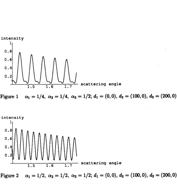
(1983).

Appendix :Figures of differential

cross

sections

Thedifferential

cross

section is aquantityobservable through actual experiments

and it is

one

of the most important quantities in the scattering theory. We here

figure the approximate values for $|f_{d}(\omega_{1}arrow\tilde{\omega};E)|^{2}$, $\omega_{1}=(1,$0), to

see

how the

intensity of scattering changes with three flux parameters $\alpha_{1}$, $\alpha_{2}$ and $\alpha_{3}$ and with

positionsofcentersdi, $d_{2}$, $d_{3}$

as

stated in Remark 1. We first consider the

case

that

the three centers $d_{1}=(0,$0),$d_{2}=(100,$0) and $d_{3}=(200,$0)

are

at

even

intervals

along direction $\omega_{1}=(1,$0), i.e., _{$|d_{12}|=|d_{23}|=d=100$}

.

The figures

are

drawn

for $|f_{d}(\omega_{1}arrow\tilde{\omega};E)|^{2}$ with E $=1$ and $4\pi/9<\gamma(\tilde{\omega};\omega_{1})<5\pi/9$

.

For example,

the scattering angle $\gamma(\tilde{\omega};\omega_{1})=\pi/2$ corresponds to the value $\pi/2=1.57\ldots$

.

on

the

horizontal axis in the figures below.

Figure 1 $(\alpha_{1}=1/4, \alpha_{2}=1/4, \alpha_{3}=1/2)$ : three coefficients do not vanish.

Figure 2 $(\alpha_{1}=1/2, \alpha_{2}=1/2, \alpha_{3}=1/2)$ : coefficient of$f_{2}(\omega_{1}arrow\tilde{\omega};E)$ vanishes.

Figure 3 $(\alpha_{1}=1/4, \alpha_{2}=(\arctan 2)/\pi$, ₀₃ $=1/2$_{) :} coefficient of$f_{3}(\omega_{1}arrow\tilde{\omega};E)$

vanishes.

Next

we

consider the

case

that $d_{3}$

moves

only alittle ffom $(200, 0)$ to $(200, 2)$

so

that three centers

are

not

on

the same line. Fluxes

are

the

same as

in the

case

of

Figure 3. Figure 4represents this

case.

Though the movement of$d_{3}$ is small, there

is remarkabledifferences between them

150

scattering angle

Figure 1 $\alpha_{1}=1/4$, $\alpha_{2}=1/4$, $\alpha_{3}=1/2;d_{1}=(0,0)$, $d_{2}=(1W, 0)$, $d_{3}=(200,0)$

scattering angle

Figure 2 $\alpha_{1}=1/2$, $\alpha_{2}=1/2$

,

$\alpha_{3}=1/2;d_{1}=(0,0)$

,

$d_{2}=(10,0)$

,

$d_{3}=(200,0)$

scattering angle

Figure

3

$\alpha_{1}=1/4$, _Q2 $=\pi^{-1}\arctan 2$, $\alpha_{3}=1/2;d_{1}=(0,0)$, $d_{2}=(100,0)$, $d_{3}=(2W, 0)$

intensity

scattering angle

Figure 4

$\alpha_{1}=1/4$, $\alpha_{2}=\pi^{-1}\arctan 2$, _{$\alpha_{3}=1/2;d_{1}=(0,0)$}, _{$d_{2}=(100,0)$}, _{$d_{3}=(20,2)$}