Japan Advanced Institute of Science and Technology
Text version
publisher
URL
http://hdl.handle.net/10119/8501
Rights
BioMedical Engineering OnLine 2006, 5:25
doi:10.1186/1475-925X-5-25 This article is
available from:
http://www.biomedical-engineering-online.com/content/5/1/25 c 2006 Gao
et al; licensee BioMed Central Ltd. This is an
Open Access article distributed under the terms
of the Creative Commons Attribution License
(http://creativecommons.org/licenses/by/2.0),
which permits unrestricted use, distribution, and
reproduction in any medium, provided the original
work is properly cited.
Open Access
Research
Stress analysis in a layered aortic arch model under pulsatile blood
flow
Feng Gao
1, Masahiro Watanabe
2and Teruo Matsuzawa*
2Address: 1Graduate School of Information Science, Japan Advanced Institute of Science and Technology, 1-1 Asahidai, Nomi, Ishikawa, 923-1292,
Japan and 2Center for Information Science, Japan Advanced Institute of Science and Technology, 1-1 Asahidai, Nomi, Ishikawa, 923-1292, Japan
Email: Feng Gao - [email protected]; Masahiro Watanabe - [email protected]; Teruo Matsuzawa* - [email protected] * Corresponding author
Abstract
Background: Many cardiovascular diseases, such as aortic dissection, frequently occur on the
aortic arch and fluid-structure interactions play an important role in the cardiovascular system. Mechanical stress is crucial in the functioning of the cardiovascular system; therefore, stress analysis is a useful tool for understanding vascular pathophysiology. The present study is concerned with the stress distribution in a layered aortic arch model with interaction between pulsatile flow and the wall of the blood vessel.
Methods: A three-dimensional (3D) layered aortic arch model was constructed based on the
aortic wall structure and arch shape. The complex mechanical interaction between pulsatile blood flow and wall dynamics in the aortic arch model was simulated by means of computational loose coupling fluid-structure interaction analyses.
Results: The results showed the variations of mechanical stress along the outer wall of the arch
during the cardiac cycle. Variations of circumferential stress are very similar to variations of pressure. Composite stress in the aortic wall plane is high at the ascending portion of the arch and along the top of the arch, and is higher in the media than in the intima and adventitia across the wall thickness.
Conclusion: Our analysis indicates that circumferential stress in the aortic wall is directly
associated with blood pressure, supporting the clinical importance of blood pressure control. High stress in the aortic wall could be a risk factor in aortic dissections. Our numerical layered aortic model may prove useful for biomechanical analyses and for studying the pathogeneses of aortic dissection.
Background
The aorta is the main blood artery that delivers blood from the left ventricle of the heart to the rest of the body, and many cardiovascular diseases, such as aortic dissec-tion, often occur on the aortic arch. It has been well estab-lished that many diseases are closely associated with the
flow conditions in the blood vessels [1] and the blood flow in the aortic arch has been widely studied in the past [2-4].
Fluid-structure interactions play an important role in the cardiovascular system. There have been many recent
stud-Published: 24 April 2006
BioMedical Engineering OnLine 2006, 5:25 doi:10.1186/1475-925X-5-25
Received: 29 December 2005 Accepted: 24 April 2006 This article is available from: http://www.biomedical-engineering-online.com/content/5/1/25
© 2006 Gao et al; licensee BioMed Central Ltd.
This is an Open Access article distributed under the terms of the Creative Commons Attribution License (http://creativecommons.org/licenses/by/2.0), which permits unrestricted use, distribution, and reproduction in any medium, provided the original work is properly cited.
ies of fluid-structure interaction in the aortic valve [5], aortic aneurysm [6], and in stented aneurysm models [7]. However the interaction between a pulsatile blood flow and the aortic wall in an aortic arch model has not yet been studied.
From the mechanical point of view, ruptures appear if the stresses acting on the wall rise above the ultimate value for the aorta wall tissue [6]. Mechanical stress plays a crucial role in the functioning of the cardiovascular system; there-fore, stress analysis is a useful tool for understanding vas-cular pathophysiology [8]. Thubrikar et al. [9] used finite element analysis to determine the stresses in an aneurysm of the aorta; they found that longitudinal stress in the bulb is the only stress that increases significantly and could be responsible for the tear in an aortic dissection. Stress analysis of the aortic arch was implemented to study the effects of aortic motion on aortic dissection [10]. The present study is concerned with the stress distribution in a layered aortic arch model with interaction between a pulsatile flow and the wall of the blood vessel.
Circumfer-ential and longitudinal stress, as well as composite stress in the wall plane, is presented.
Methods
Geometry and wall properties
The radius of the arch was set at 30 mm [11] and the diameter of the vessel was assumed to be uniform (24 mm). The average diameter of the aorta is 20–25 mm [12]. The thickness of the whole wall was chosen to be 2 mm according to the characteristics of various types of blood vessels in [13]. The arch angle a is measured at the circumference of the median longitudinal cross-section, and ranges from 0° and 180° (Fig. 1), so that the wall position of the arch, as denoted by the arch angle, can be discussed.
An average thickness ratio of intima/media/adventitia of 13/56/31 for arteries was observed in Schulze-Bauer's studies [14]. The thickness ratio of media/adventitia is 2/ 1 in the computational model for the arterial wall pre-sented by Driessen et al. [15]. In this three-layered wall model, the intima/media/adventitia thickness ratio was The finite element model of the aortic arch
Figure 1
The finite element model of the aortic arch. The branches of the arch were neglected as a first order approximation.
set to 1/6/3. Therefore, the thicknesses of the intima, media, and adventitia were ti = 0.2 mm, tm = 1.2 mm, and
ta = 0.6 mm, respectively.
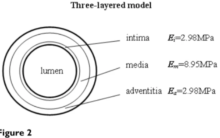
In Mosora's experiments [16], the Young's modulus of the thoracic ascending aorta was 2 MPa to 6.5 MPA. In vivo, the surrounding connective tissue and muscle can support the aortic arch. In this study, the aortic arch is a self-sup-porting structure. The maximum E = 6.5MPa was chosen for the Young's modulus of the aorta wall. Xie et al. [17] performed bending experiments and showed the Young's modulus of the inner layer (intima and media) was three to four times larger than that of the outer layer (adventi-tia), and we can deduce from Fischer's experimental data [18] that the Young's modulus of the intima is smaller than that of the media. In the present study, the Young's modulus of the media is assumed to be three times larger than that of the adventitia and the intima. Since the mean Young's modulus of the vessel wall across whole wall vol-ume is invariable, we assvol-ume that the Young's modulus of each layer is in inverse proportion to the area of the layer in the cross section. Based on the area equation, the Young's modulus of the intima, media, and adventitia lay-ers is 2.98MPa, 8.95MPa, and 2.98MPa respectively. Fig. 2 shows the three-layered aortic wall.
Fluid-structure interaction
Fig. 1 shows the circulatory system; the blowup is the FEM model of the aorta. The finite element analysis model of the aorta was made of 38400 eight-node brick elements for the solid domain and 26880 eight-node brick ele-ments for the fluid domain. There are 20 eleele-ments through the thickness of the aorta wall.
In a fluid-structure interaction problem, fluid affects struc-ture and strucstruc-ture also affects fluid. In this study, the pro-cedure is based on the loose coupling of three fields of
problems: the flow, the elastic body, and the mesh move-ment – that is, CFD (computational fluid dynamics), CSD (computational structural dynamics), and CMD (compu-tational mesh dynamics) procedures [19].
The FSI (Fluid Structure Interaction) algorithm treats the equations that solve the fluid problem, the structural problem, and the re-meshing problem by a staggered approach; that is to say, the algorithm solves the equa-tions in sequence. The overall computational procedure adopted to solve FSI problems is depicted in Fig. 3. Oper-atively, a ALE (Arbitrary Lagrangian Eulerian) algorithm is used which seeks, at each step increment, the convergence of the three blocks of equations, fluid (CFD), solid (CSD) and mesh movements (CMD). These must then converge altogether before a new step is initiated. The detailed equations are described in the Appendix.
The code Fidap (Fluent Inc., Lebanon, NH) was used to carry out the simulation. Bar-Yoseph et al. [20] gave many examples to demonstrate the validity of the method used in this study. Marzo et al. [21] also used the same method to do a FSI simulation and got excellent results.
Typically, 160–190 iterations were required per time step to reduce the residuals. The numerical convergence is a relative change in the solution from one iteration to the next of less than 0.0001.
Circumferential stress is the normal stress that points along the tangent direction to a cross-section circle in the cross-section plane. Longitudinal stress is the normal stress that points in the direction of the axis of the vessel. Composite stress is the composition of the circumferen-tial stress vector and the longitudinal stress vector, which is the resultant stress in the wall plane.
Boundary condition and properties of fluid
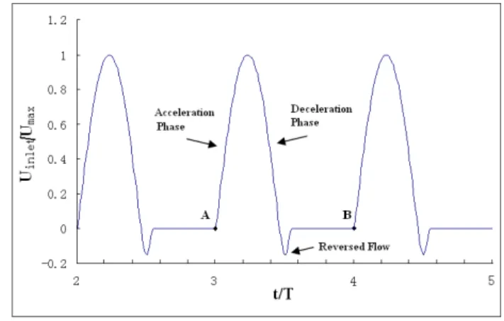
The boundary conditions are time-dependent. At the aor-tic inlet, a flat flow velocity profile was used together with a pulsatile waveform based on experimental data reported by Pedley [22]. This waveform is shown in Fig. 4. The assumption of a flat velocity profile at the aortic inlet is justified by in vivo measurements using hot film ane-mometry on various animal models, which have demon-strated that the velocity profile distal to the aortic valve are relatively flat [23]. The Reynolds number for blood flow is approximately 4000 in the aorta [24]. In our calculations, the Reynolds number is fixed at Re = 4000 based on the inlet velocity at peak systole of the cardiac cycle. There is pressure both at the inside and the outside of the blood vessel and the pressure difference between the inside and the outside of the blood vessel tends to deform the blood vessel [24]. This study was concerned mainly with the effect of the relative pressure on the wall stress. At the aor-Three-layered models
Figure 2
Three-layered models. The Young's modulus of layers is
tic outlet, a zero pressure condition was applied. The sur-face of the inlet was fixed. The outer edge of the outlet was constrained in the axial direction and permitted to move in the other directions. There was no constraint for the other parts of the aorta model.
The simulation reached nearly steady-state oscillation after approximately the third cycle. The fourth cycle was used as the final periodic solution and it is presented in this paper.
The fluid is Newtonian with a density of 1050 kg/m3 and a viscosity of 0.0035 Pa s. Blood is essentially a suspen-sion of erythrocytes in plasma and shows anomalous vis-cous properties at low velocities. However, the Newtonian assumption is considered acceptable since minor differ-ences in the basic flow characteristics are introduced through the non-Newtonian hypothesis [25].
Results
Result pressure
The pressure waveform at the inlet corresponding to the inlet velocity was extracted from result data (Fig. 5). We see the pressure rises above zero (1330Pa) at the start of systole during the accelerative phase and then becomes negative at peak systole, reaching a minimum value (-1100Pa) at the max reverse flow. There is a transient increase in pressure after the max reversed flow phase. A negative pressure represents the decelerative phase of the aortic flow.
Fig. 6 shows the variations of pressure along the arch at centerline during the cardiac cycle. The variations of pres-sure as a function of time are similar to the results shown in Fig. 5. Positive pressure values decrease along the arch portion.
Variations of stresses along arch during cardiac cycle
Tears and dissections usually involve the outer wall of the arch [26], so the stress distribution in the outer wall was investigated. Fig. 7 presents the variations of circumferen-Inlet velocity profile
Figure 4
Inlet velocity profile. t is the time, T is the total time in
one cycle. For the final run, the cardiac cycle starts at A and ends at B.
Strategy of the computational procedure
Figure 3
tial stress and longitudinal stress on the outer wall along the arch portion during the cardiac cycle. The stresses are averaged across the aortic wall thickness.
The circumferential stress on the outer wall initially increases at the start of systole and then decreases below zero during the deceleration phase. After the reverse flow, there is a transient increase in mean circumferential stress.
The circumferential stress is higher in the ascending por-tion than in the descending porpor-tion. The variapor-tion of the mean circumferential stress in the outer wall of the arch is similar to the variation of the pressure at the arch outer wall.
Longitudinal stress initially increases at the acceleration phase of systole, then deceases, and then increases a little at the reverse flow. The high stress regions along the arch are at the entrance to the ascending portion, the top of the arch, and the distal end of the arch.
Since the stress in the acceleration phase is high, a tran-sient time t/T = 0.12 in the middle of the acceleration phase was selected to characterize the variations of stresses along the arch in detail. The circumferential stress and the longitudinal stress, as well as the composite stress along the arch at selected transient times, are shown in Fig. 8. The circumferential stress decreases along the arch. The longitudinal stress along the arch gets peak values at the entrance to the ascending portion, the top of the arch, and the distal end of arch. The composite stress decreases, with a peak at the top of the arch along the arch portion.
Variations of stresses across the wall
Four positions, a = 22.5°, a = 67.5°, a = 112.5°, and a = 157.5°, were selected in the arch portion to illustrate the variation of stresses across the wall.
Pressure at centerline as a function of the function of arch angle a and time t/T
Figure 6
Pressure at centerline as a function of the function of arch angle a and time t/T. End diastole is at t/T = 4.0. Angle a
represents the wall position in the arch portion.
Pressure waveform at inlet corresponding to inlet velocity
Figure 5
Pressure waveform at inlet corresponding to inlet velocity.
The variations of circumferential, longitudinal, and com-posite stress across the three-layer model wall at four posi-tions at systolic acceleration (t/T = 3.12) are shown in Fig. 9. The stress is much higher in the media layer than in the intima and adventitia layers.
Discussion
We have simulated the complex mechanical interaction between blood flow and wall dynamics by means of com-putational coupled fluid-structure interaction analyses and shown the results for mechanical stress in the layered Variation of circumferential and longitudinal stress at arch outer wall as a function of the function of arch angle a and time t/T
Figure 7
Variation of circumferential and longitudinal stress at arch outer wall as a function of the function of arch angle a and time t/T. (a) Circumferential stress variation. (b) Longitudinal stress variation. End diastole is at t/T = 4.0. Angle a
aortic arch model. The composite stress in the aortic wall plane is high at the ascending portion and along the top of the arch and is higher in the media than in the intima and adventitia across the wall thickness.
Circumferential stress was considered an important parameter for mechanosensitive receptors. Under a pres-sure P, the circumferential and longitudinal stresses in a cylinder of thickness t and radius R are PR/t and PR/2t,
respectively [9]. Our resulting pressure waveform at the inlet in the present study agrees with the results in Tyszka's [27] paper. This demonstrates that circumferential stress depends on the systolic blood pressure. Furthermore, this explains the fact that 70–90% of patients with aortic dis-section have high blood pressure [26,28-30] and supports the clinical importance of blood pressure control in reducing the risk of tearing and rupturing in aortic dissec-tion.
The pressure P decreased along the arch portion, and the radius R and thickness t did not change very much. How-ever, the longitudinal stress depicted in Fig. 8(b) along the arch gets peak values at the entrance to the ascending por-tion, the top of the arch, and the distal end of arch, so the variation would be unpredictable using PR/2t; thus, the shape of the arch and fluid force may play crucial roles in aorta mechanics. Similar work on the stress distribution on the aortic arch has been presented by Beller et al. [10], in which circumferential and longitudinal stress were found to be maximum at the top of the arch. Unfortu-nately, they only used a load condition of 120 mmHg luminal pressure and the pulsatile flow condition was not considered. In recognizing the influential effects of pulsa-tile flow in the aortic mechanism, a more realistic wall stress distribution was simulated in our coupled model. Bellers et al. [10] included branch vessels in their model. Our study was concerned mainly with the effects of the aortic arch on stress distribution. Therefore, the branches along the top of the aortic arch were not included in the model.
Thubrikar et al. [9] have proposed that longitudinal stress could be responsible for transverse tears in the aortic dis-section. Roberts [26] reported that in 62% of patients the tear is located in the ascending aorta, usually about 2 cm cephalad to the sinotubular junction. This means the loca-tion is about a = 0°, at the entrance to the ascending por-tion of the arch. After the ascending aorta, about 20% of tears are at the aortic isthmus portion [26], which is near the top of the arch. In the present study, the longitudinal stress achieved peak values at the entrance to the ascend-ing portion and the top of the arch. Yet, the longitudinal stress also peaked in the distal end of the arch, and tears do not often occur at this location.
Composite stress was high at the entrance to the ascend-ing portion and at the top of the arch; the value at the entrance to the ascending portion was a little higher. The location of this high composite stress value is consistent with the tear locations identified in the Roberts report [26]. This implies that both circumferential and longitudi-nal stress may contribute to the tear in an aortic dissection and high composite stress in the aortic wall could be a risk factor for tears in aortic dissections.
Stress distribution on the outer wall along the arch portion
Figure 8
Stress distribution on the outer wall along the arch portion. (a) Circumferential stress distribution. (b)
Variation of the stresses across the wall at four positions (a = 22.5°, a = 67.5°, a = 112.5°, and a = 157.5°) at selected time of systolic acceleration (t/T = 3.12)
Figure 9
Variation of the stresses across the wall at four positions (a = 22.5°, a = 67.5°, a = 112.5°, and a = 157.5°) at selected time of systolic acceleration (t/T = 3.12).
The stress variation across wall thickness was due to the non-homogeneous wall properties. Our results showed that the stress was highest in the media across the aortic wall thickness and this agreed with the results of Maltzahn et al. [31], that the media was subject to much higher stresses. These results might partially explain why the location of the dissection is in the aortic media [26]. Previous studies [32,33] examined the properties of the aorta and showed the aortic wall is anisotropic. The smooth muscle cells in aortic wall were torn loose from their attachments to each other and to the adjacent elastin [33], so the dissection may propagate rather than tearing back through the intima or out through the adventitia. Residual stresses can affect stress distribution through the arterial wall. Circumferential stress distributions includ-ing residual stress have shown decreased inner wall stress [34], which may be induced by the negative value of resid-ual stress in inner side of wall [17]. The residresid-ual stress is high in the outer side of media and positive at adventitia [17] and this may increase the stress at the outer side of media and at adventitia.
The aortic arch model used here only partially simulated the real situation because it neglected the effect of the branches of the arch [3,4] and the aortic arch's non-planarity [35]. Because this was an initial attempt; the model was purposely kept simple in order to give an insight into the stress distribution on the aortic arch with interaction between a pulsatile flow and the wall. Further-more, more than 80% of tears and dissections are at the aorta, not at branches of the arch [26,36]. In the future investigations, the branches will be added to the model. The mechanical properties of arteries have been reported extensively in the literature. The type of nonlinearity is a consequence of the curvature of the strain-stress function, which shows that an artery becomes stiffer as the distend-ing pressure increases. Horsten et al. [37] showed that elasticity dominates the nonlinear mechanical properties of arterial tissues. In numerical simulation of the biome-chanics in arteries [6-8,10], the wall was assumed to be an elastic constitutive model. Of course, a non-linear consti-tutive model could provide more biological aspects of the biomechanics. In future work we plan to implement the nonlinear properties of aortic wall within the code by means of user-subroutines.
Conclusion
In summary, our analysis indicates that circumferential stress in the aortic wall is directly associated with blood pressure, supporting the clinical importance of blood pressure control. High stress in the aortic wall could be a risk factor for tearing in aortic dissections. This numerical layered aortic model may prove useful for biomechanical
analyses and for studying the pathogeneses of aortic dis-section.
Appendix
Detailed equations of FSI algorithm
1. Computational Fluid Dynamics (CFD)
The ALE (Arbitrary Lagrangian Eulerian) form of the Navier-Stokes equations are used to solve for fluid flow for FSI problems. After spatial discretization by the finite element method, the Navier-Stokes equations are expressed in the ALE formulation:
Ma + N(v - )v + Dv - Cp = f in F Ω(t) (1)
CT v in F Ω(t) (2)
where M represents the fluid mass matrix; N, D, and C are, respectively, the convective, diffusive, and divergence matrices; f is an external body force; vectors a, v, and p contain the unknown values of acceleration, velocity, and pressure, respectively; is the mesh velocity, calculated using Eq. (13) in CMD; and F Ω(t) is the moving spatial domain upon which the fluid is described.
The following compatibility conditions are imposed on the interface between fluid and structure:
where (F) indicates values related to nodes placed in the fluid; (S) indicates values related to the nodes placed in the structure; and IΓ(t) is the interface between fluid and structure at time t. s v and sa are calculated at the previous iteration loop in CSD.
The fluid velocity and pressure field are solved after initial conditions, boundary conditions and compatibility con-ditions are imposed on the fluid domain. For calculating the traction at the interface between fluid and structure vectors a, v, and f are decomposed into:
where (U) indicates values related to nodes on the velocity boundary, (I) indicates values related to the fluid nodes on the interface between fluid and structure, and the sym-bol (-) denotes the prescribed values. The load applied by the fluid on the structure along the interface between fluid and structure is obtained according to partitioned Eq. (1):
ˆv ˆv F S F S I t v v a a = = on Γ
( )
( )
3 aT={
Fa,Ua a,I}
, vT={
Fv,Uv v,I}
, fT={
Ff,Uf f,I}
( )4M, N, D, C, a, v, and p are known values solved in the
pre-vious process in this equation. The traction is imposed on the structure in CSD.
2. Computational Structural Dynamics (CSD)
The overall structural behavior is described by the matrix equation:
s M s a+s K s d= + - σ f in sΩ(t) (6)
where S M and S K are the structural mass and nonlinear stiffness matrices; is the external body force vector; , calculated using the Eq. (5) in CFD, is the traction applied by the fluid on the structure along the interface; σ
f is the force due to the internal stresses at the most
recently calculated configuration; S d is the vector of incre-ments in the nodal point displacement; S a is the vector of nodal point acceleration; s Ω(t) is the structure domain at time t. and σ f are equal to zero in this study. The
equa-tion of moequa-tion can be integrated and the displacement, velocity, and acceleration vectors can be calculated. The displacement at the interface between fluid and struc-ture can be calculated and the surface location is updated: I d = s d on I Γ(t) (7)
The mesh displacement can be obtained at the interface between fluid and structure:
= I d on I Γ(t) (8)
The mesh displacement is imposed at the interface between fluid and structure in CMD.
3. Computational mesh dynamics (CMD)
where is the stiffness matrix, and is the mesh dis-placement vector defined by
where s the mesh position vector, and t ref is the refer-ence time. Eq. (9) can be rewritten in a partitioned form as
On the interface between fluid and structure, the mesh displacement given by Eq. (8) from CSD is imposed. So we obtain
which shows that the fluid mesh motion is driven by the elastic body motion. This equation, together with the other boundary condition, was solved for the fluid mesh displacement.
The fluid mesh displacement was solved and the mesh geometry was updated. The mesh velocity field can be obtained:
The mesh velocity is imposed in CFD.
Acknowledgements
This research is conducted as a program for the "Fostering Talent in Emer-gent Research Fields" in Special Coordination Funds for Promoting Science and Technology by the Japanese Ministry of Education, Culture, Sports, Sci-ence and Technology.
References
1. Moayeri MS, Zendehbudi GR: Effects of elastic property of the
wall on flow characteristics through arterial stenoses. J
Bio-mech 2003, 36:525-535. I t S f It S f I t Sf Iˆd Iˆd ˆ K ˆd ˆ ˆ ˆ d=R
( )
t −R( )
tref( )
10 ˆ R FF FI IF II F I ˆ ˆ ˆ ˆ ˆ ˆ K K K K d d 0 0 = ( )
11 FFK dˆ ˆF = −FIK dˆ ˆI( )
12 ˆ ˆ / v=d(
t−tref)
( )
13Publish with BioMed Central and every scientist can read your work free of charge "BioMed Central will be the most significant development for disseminating the results of biomedical researc h in our lifetime."
Sir Paul Nurse, Cancer Research UK Your research papers will be:
available free of charge to the entire biomedical community peer reviewed and published immediately upon acceptance cited in PubMed and archived on PubMed Central yours — you keep the copyright
Submit your manuscript here:
http://www.biomedcentral.com/info/publishing_adv.asp
BioMedcentral 2. Endo S, Sohara Y, Karino T: Flow patterns in dog aortic arch
under a steady flow condition simulating mi-systole. Heart
Vessels 1996, 11:180-191.
3. Shahcheraghi N, Dwyer HA, Cheer AY, Barakat AI, Rutaganira T:
Unsteady and three-dimensional simulation of blood flow in the human aortic arch. J Biomech Eng 2002, 124:378-387.
4. Kim T, Cheer AY, Dwyer HA: A simulated dye method for flow
visualization with a computational model for blood flow. J
Biomech 2004, 27:1125-1136.
5. Hart JD, Peters GWM, Schreurs PJG, Baaijens FPT: A
three-dimen-sional computational analysis of fluid-structure interaction in the aortic valve. J Biomech 2003, 36:103-112.
6. Di Martino ES, Guadagni G, Fumero A, Ballerini G, Spirito R, Biglioli P, Redaelli A: Fluid-structure interaction within realistic
three-dimensional models of the aneurysmatic aorta as a guidance to assess the risk of rupture of the aneurysm. Med Eng Phys
2001, 23:647-655.
7. Li Z, Kleinstreuer C: Blood flow and structure interactions in a
stented abdominal aortic aneurysm model. Med Eng Phys 2005, 27:369-382.
8. Giannakoulas G, Giannoglou G, Soulis J, Farmakis T, Papadopoulou S, Parcharidis G, Louridas G: A computational model to predict
aortic wall stresses in patients with systolic arterial hyper-tension. Med Hypotheses 2005, 65:1191-1195.
9. Thubrikar MJ, Agali P, Robicsek F: Wall stress as a possible
mech-anism for the development of transverse intimal tears in aor-tic dissections. J Med Eng Tech 1999, 23:127-134.
10. Beller CJ, Labrosse MR, Thubrikar MJ, Robicsek F: Role of aortic
root motion in the pathogenesis of aortic dissection.
Circula-tion 2004, 109:763-769.
11. Mori D, Tsubota K, Wada S, Yamaguchi T: Concentrated High
Shear Stress due to the Torsion of the Aortic arch and Development of the Aortic Aneurysm. In ASME Summer
Bioen-gineering Conference Florida, USA. 23–30 June 2003
12. Engel N: Abdominal aortic aneurysm and low back pain. Dynamic Chiropractic 1996, 14(16):.
13. Ganong WF: Review of Medical Physiology Lange Medical Publications; 1963.
14. Schulze-Bauer CA, Morth C, Holzapfel GA: Passive biaxial
mechanical response of aged human iliac arteries. J Biomech
Eng 2003, 125:395-406.
15. Driessen NJB, Wilson W, Bouten CVC, Baaijens FPT: A
Computa-tional Model for Collagen Fibre Remodeling in the Arterial Wall. J Theor Biol 2004, 226:53-64.
16. Mosora F, Harmant A, Bernard C, Fossion A, Poche T, Juchmes J, Cescotto S: Modelling the arterial wall by finite elements. Arch Int Physiol Biochim Biophys 1993, 101:185-191.
17. Xie J, Zhou J, Fung YC: Bending of blood vessel wall:
stress-strain laws of the intima-media and adventitial layers. J
Bio-mech Eng 1995, 117:136-145.
18. Fischer EI, Armentano RL, Pessana FM, Graf S, Romero L, Christen AI, Simon A, Levenson J: Endothelium-dependent arterial wall
tone elasticity modulated by blood viscosity. Am J Physiol Heart
Circ Physiol 2002, 282:389-394. 19. Fidap Theory Manual, Fluent Inc .
20. Bar-Yoseph PZ, Mereu S, Chippada S, Kalro VJ: Automatic
moni-toring of element shape quality in 2-D and 3-D computa-tional mesh dynamics. Computacomputa-tional Mechanics 2001, 27:378-395.
21. Marzao A, Luo XY, Bertram CD: Three-dimensional collapse
and steady flow in thick-walled flexible tubes. Journal of Fluid
and Structures 2005, 20:817-835.
22. Pedley TJ: The Fluid Mechanics of Large Blood Vessels Cambridge Uni-versity Press; 1980.
23. Nerem RM: Vascular fluid mechanics, the arterial wall, and
atherosclerosis. J Biomech Eng 1992, 114:274-282.
24. Ku DN: Blood flow in arteries. Annu Rev Fluid Mech 1997,
29:399-434.
25. Liepsch D, Moravec S, Baumgart R: Some flow visualization and
laser-doppler velocity measurements in a true-to-scale elas-tic model of a human aorelas-tic arch – a new model technique.
Biorheology 1992, 29:563-580.
26. Roberts WC: Aortic dissection: anatomy consequences and
causes. Am Heart J 1981, 101:195-214.
27. Tyszka JM, Laidlaw DH, Asa JW, Silverman JM: Three-dimensional,
time-resolved (4D) relative pressure mapping using mag-netic resonance imaging. J Magn Reson Imaging 2000, 12:321-329.
28. Jamieson WRE, Munro AI, Miyagishima RT, Allen P, Tyers GFO, Gerein AN: Aortic dissection: early diagnosis and surgical
management are the keys to survival. Can J Surg 1982, 25:145-149.
29. Desanctis RW, Doroghazi RM, Austen WG, Buckley MJ: Aortic
dis-section. N Engl J Med 1987, 317:1060-1067.
30. Slater EE, Desanctis RW: The clinical recognition of dissecting
aortic aneurysm. Amer J Med 1976, 60:625-633.
31. Maltzahn WWV, Warriyar RG, Keitzer WF: Experimental
meas-urements of elastic properties of media and adventitia of bovine carotid arteries. J Biomech 1984, 17:839-848.
32. Dobrin PB: Mechanical properties of arteries. Physiol Rev 1978,
58:397-460.
33. Maclean NF, Dudek NL, Roach MR: The role of radial elastic
properties in the development of aortic dissections. J Vasc
Surg 1999, 29:703-710.
34. Peterson SJ, Okamoto RJ: Effect of residual stress and
heteroge-neity on circumferential stress in the arterial wall. J Biomech
Eng 2000, 122:454-456.
35. Mori D, Yamaguchi T: Computational mechanical analysis of
blood flow in the human aortic arch with complex 3-D con-figuration – a combined effect of the torsion of the aorta and its branches. In 2001 Bioengineering Conference Volume 50. ASME;
2001:741-742.
36. Hume DM, Porter RR: Acute dissecting aortic aneurysms. Sur-gery 1963, 53:122-154.
37. Horsten JB, van Steenhoven AM, van Dongen AA: Linear
propaga-tion of pulsatile waves in viscoelatic tubes. J Biomech 1989, 22:477-484.