Research Development of 4Dimensional Data Assimilation System using a Coupled Climate Model and Construction of Reanalysis Datasets for

Research Development of 4-Dimensional Data

Assimilation System using a Coupled Climate Model and

Construction of Reanalysis Datasets for Initialization

Project Representative

Toshiyuki Awaji

Authors

Toshiyuki Awaji

, Nozomi Sugiura

, Takashi Mochizuki

Shuhei Masuda

,

Toru Miyama

, Nobuhiro Ishida

, Hiromichi Igarashi

, Yoichi Ishikawa

,

Kazutoshi Horiuchi

, Nobumasa Komori

, Yuji Sasaki

and Yoshihisa Hiyoshi

1 Frontier Research Center for Global Change 2 Department of Geophysics, Kyoto University 3 Advanced Earth Science & Technology Organization 4 NEC Informatec Systems, Ltd.

5 The Earth Simulator Center

Improvements of a climate model used for 4-dimensional variational coupled data assimilation have been conducted with a particular emphasis on a new diagnostic scheme for determining the marine stratocumulus (SCu) cloud cover that plays a cru- cial role in the atmosphere-ocean feedback in the tropics. When the new scheme is applied to a coupled GCM, the SCu cloud cover becomes more representative in both spatial and seasonal variations, and SST values to the west of continents in sub- tropical areas display weakened warm biases and more realistic seasonal cycles resulting from the modification of the down- ward shortwave radiation flux at the sea surface. Furthermore, the new scheme introduces both local and large-scale improve- ments in model climatology over low-and mid-latitude regions. In the eastern Pacific, for example, a shallow meridional cir- culation across the equator is excited, and the strength and location of the intertropical convergence zone (ITCZ) and the sea- sonal cycle of equatorial SST become more realistic. These results are beneficial to better representation of climate variabili- ties and more reliable predictions by coupled data assimilation.

Keywords: Marine Stratocumulus Cloud Scheme, Coupled GCM and Data Assimilation, Climatological Features, Variability and Predictability

1. Introduction

In our research project, we take up the challenge of devel- oping a leading-edge 4D-VAR coupled data assimilation system on the Earth Simulator, with the aim to better repre- sent the dynamical state of climate variability and thereby construct a comprehensive reanalysis dataset offering greater information content and forecast potential for climate events such as the monsoon, El Niño and Southern Oscillation (ENSO) phenomena. So far we have succeeded in construct- ing such a 4D-VAR coupled data assimilation system and applied it to the representation of the climatological seasonal state of the global environment.

In order to enhance the physical performance of our cou- pled data assimilation system, further improvements of atmos- phere-ocean-sea ice-land surface model used in the system on

the Earth Simulator (CFES) are required, because levels of performance of any 4D-VAR approach depend greatly on those of models used. For this reason, we have made further modifications of CFES. In doing so, our attention is directed to the development of a diagnostic scheme for determining the marine stratocumulus (SCu) cloud cover that plays a cru- cial role in the atmosphere-ocean feedback in the tropics.

It is well--known that coupled general circulation models (GCMs) generally simulate strongly biased sea surface tem- peratures (SST) that result in excessively warm water to the west of continents in subtropical regions [Mechoso et al. 1995; Dai 2005]. One of the major reasons for this bias is thought to be the poor reproducibility of marine Scu, due to inadequate physical parameterization and the coarse resolu- tion of GCMs [e.g., Bretherton et al. 2004]. Along the west

coast of South America, for example, an unrealistically enhanced downward solar radiation flux at the sea surface resulting from poorly simulated SCu overheats the upper ocean. The ocean thermal condition in that region seems to have a crucial effect on the location of the intertropical con- vergence zone (ITCZ) and the strength of the equatorial cold tongue [e.g., Philander et al. 1996].

Some recent studies have improved the physical parame- terization [Bachiochi and Krishnamurti 2000; Teixeira and Hogan 2002]. However, SCu is still poorly simulated in most GCMs in use today [Siebesma et al. 2003]. These stud- ies demonstrated that the atmospheric fields were substan- tially modified by marine SCu variability and highlighted the importance of slow upward transport of heat moisture and momentum by shallow convection [Wang et al. 2004b].

In line with these advances, the purpose of the present study is to develop a simple and effective diagnostic calcu- lation scheme for marine SCu, in order to improve the sim- ulated climate features of the lower troposphere and reduce the warm SST biases detected along the west coasts of con- tinents in subtropical regions in coupled GCMs (CGCMs). This is quite important for improved estimates of seasonal to interannual (S-I) phenomena by the coupled data assimi- lation. The calculation scheme is based on Slingo [1987] with modifications introduced on the basis of recent obser- vational and modeling studies. The salient features of the new scheme in the present study are the seasonal and spatial variabilities of the regression coefficients and the considera- tion of the slow upward transport of heat, moisture and momentum in sub-cloud layers accompanying the SCu component. Here, the reproducibility of the SCu and of related atmosphere-ocean climate systems in CGCMs will be examined.

2. Simple diagnostic scheme for marine stratocumulus The atmosphere-ocean coupled model employed here is the Coupled model for the Earth Simulator (CFES), which is composed of the AGCM for the Earth Simulator (AFES) [Ohfuchi et al. 2004] and the Ocean-sea Ice GCM for the Earth Simulator (OIFES) [e.g., Komori et al. 2005]. The AFES is based on the AGCM by the Center for Climate System Research/ National Institute for Environmental Studies (CCSR/NIES). The radiation code has been modified using MstrnX [Nakajima et al. 2000; Sekiguchi et al. 2003]. The OIFES component was developed from version 3 of the Modular Ocean Model (MOM3) produced by the Geophysical Fluid Dynamics Laboratory and the sea ice model of the International Arctic Research Center [Hibler 1980].

Two cloud schemes have already been used in the AFES component. One of these is the deep convective parameteri- zation based on Arakawa and Schubert [1974] and Moorthi and Suarez [1992]. The other treats large-scale condensa-

tion using the method of Le Treut and Li [1991], in which only the total water content is prognostically calculated at each grid point, and other related values such as liquid water content and cloud cover are diagnostically calculated. A shallow convection scheme is not implemented in the AFES model.

In addition to these two cloud schemes, a diagnostic scheme for marine SCu cloud cover is developed as follows. Since a well-correlated relationship is observed between the coverage of low level clouds and the stability of atmosphere at greater altitudes [Philander et al. 1996], the SCu cloud cover is parameterized using a linear regression equation based on the atmospheric stability just above a given layer as,

where c, θ and p are cloud cover, potential temperature and air pressure, respectively. The suffix k denotes the vertical grid point from the surface to the top of the atmosphere in sigma coordinates. The spatio-temporal dependence of the regression coefficients α and β is determined here by statis- tical estimation using observational datasets, whereas these coefficients were set to constant values in Slingo [1987]. The resolution of the regression coefficients is horizontally the same as the T42 spectral model, vertically 4 layers from 1000 hPa to 700 hPa at 75 hPa intervals, and temporally 12 months. Although the vertical resolution seems to be too coarse to represent sharp temperature inversions realistically, it is suitable to simulate SCu in the AGCM of CFES model, since the vertical resolutions are almost equal in both cases over the lower troposphere and the sharpness of the vertical gradient of potential temperature estimated from ERA40 at 75 hPa intervals is thought to be similar to that of the AFES simulator (24 layers in sigma coordinates). The considera- tion of the spatial distribution and seasonality of SCu is of major importance here, since the present scheme aims to reflect the strong spatial and seasonal changes observed in the SCu cloud cover. The atmospheric stability is calculated from ERA40, and the cloud cover data are taken from the International Satellite Cloud Climatology Project (ISCCP) D2. Monthly mean global datasets for 17 years (1984–2000) on a 2.5° × 2.5° grid are used in the present study. As we intend to achieve a realistic climate simulation focusing not on individual SCu systems but also on the monthly mean features of the SCu, it is deemed appropriate to use the monthly mean data.

The shorter timescale (e.g., daily or 6hourly) variations of low level clouds depend strongly on synoptic disturbances rather than on large-scale temperature inversions, even on the west coasts of continents, while longer timescale (e.g., monthly) variations are closely related to the strength of the temperature inversion [Philander et al. 1996].

The cloud water mixing ratio q_cldwis represented as,

where q_satis the saturation specific humidity. The parameter γ is set to be 0.01 in the present study. Note that qcldw no longer exceeds the total water mixing ratio at each grid point.

In order to represent the marine SCu cover near the west coasts of continents in subtropical regions, this diagnostic scheme is applied to heights below 700 hPa only and in sit- uations for which the layer just above the strong stable layer is sufficiently dry (i.e., the relative humidity is less than 0.6). The latter criterion corresponds to the existence of large-scale subsidence above the stable layer and the simu- lation results display few differences even if the threshold of the relative humidity is set to a slightly different value (e.g., from 0.5 to 0.8). Note that the SCu cloud cover is set to zero at a grid point where the coefficient α is negative, or where deep convective clouds are produced by the Arakawa-Schubert scheme. It should also be noted that either the cloud formation calculation (LTL91) or the above diagnostic scheme is used in conjunction with the deep con- vection scheme at each grid point. Further, the scheme is used when conditions related to the existence of SCu are satisfied, while the LTL91 formulation is used when these conditions are not satisfied.

Another feature of this scheme is the consideration of the slow upward transport of heat, moisture and momentum associated with the presence of SCu [Wang et al. 2004b]. In the absence of strong large-scale convergence near the sur- face, such upward motion is known as shallow convection. Here, the upward transport of heat, moisture and momentum from the top of the mixed layer to the bottom of the strong temperature inversion where the SCu are generated is simu- lated by controlling the strength of the vertical diffusion coefficient. For points below the stable layers, if the moist static energy becomes larger than that at the height where the SCu exists, the vertical diffusion coefficient K is aug- mented by K_sc(giving K + K_sc). The parameter K_scis set to be 10 m²s^–1in the present study. One of the reasons why a simple parameter Ksc is used for the representation of slow upward motion in the present study is the coarse vertical res- olution of the model. In recent modeling studies, shallow convection is usually represented by using the strength of the mass flux [e.g., Bretherton et al. 2004]. Note that modifica- tions to the vertical diffusion coefficient are not made below 900 hPa to prevent the mixed layer from becoming too deep. It should also be noted that shallow convection taking place without low level clouds is not represented in the present model, although such convection with SCu present is repre- sented by K_sc. This is clearly one limitation of the present scheme.

3. Coupled GCM simulation

An investigation is made into the effects of the above diagnostic scheme on the results of a CGCM simulation, focusing on the large-scale modifications of the lower tropo- sphere and SST field and their seasonal variations. The reso- lution of the OIFES is 1° in latitude and longitude and it uses 36 layers in depth. The initial conditions taken to represent the atmosphere are the results of a 2-year AFES simulation with the climatological SST and those for the ocean are the result of a 15-year OIFES simulation with the climatological atmospheric conditions taken from the NCEP/NCAR reanalysis dataset. The CFES is integrated for 12 years and the results of the last 10 years are derived from three experi- ments (the SCu scheme (CTL-C), the SCu scheme with annually averaged regression coefficients (ANL-C) and a no-SCu scheme (NoSC-C)) and are compared .

3.1 Large--scale modification of the eastern Pacific by SCu Large-scale improvement of the simulated climatological atmosphere-ocean system is clearly found in the eastern Pacific. The cloud cover west of continents is significantly improved in the CTL-C scheme (Fig. 1). The vertical struc- tures of SCu off Peru in the CGCM simulation are very simi- lar to those of the AGCM simulation (not shown), although the mixed layer clouds in the CGCM simulation are shifted slightly eastward (trapped near the coastal region) compared to the AGCM situation.

The downward shortwave radiation flux at the sea surface is also considerably improved (Fig. 2a). Near the continents, both in the Californian and Peruvian regions, the downward shortwave radiation flux is reduced due to the enhanced SCu along the coastlines. As a result, warm biased SST values are suppressed along the west coasts of continents, where strong development of SCu clouds takes place (Fig. 2b). It should be noted that the short wave radiation flux is reduced in the CTL-C scheme (Fig. 2a), although the cloud water mixing ratio is also reduced (Fig. 1). This curious feature is explained by differences in the amplitudes of the diurnal cycles between the CTL-C and NoSC-C simulations. Since the amplitude of the diurnal cycle in the CTL-C scheme is larger (not shown), the cloud water mixing ratio here is weakened during nighttime but is enhanced during daytime as compared with the NoSC results, while the daily averaged value in the CTL-C data is clearly weakened. Therefore, downward propagation of short wave radiation is blocked more effectively by low level clouds enhanced in daytime, and is reduced at the sea surface in the CTL-C scheme. Note that the qualitative characteristics of the diurnal cycle of low level cloud cover (maximum in early morning and minimum in the evening) is still consistent with the observational results [e.g., Bretherton et al. 2004]. Far from the continents, on the other hand, the simulated SST becomes warmer due

Above the SCu, on the contrary, anomalous southward winds are found across the equator and an anomalous diver- gence is formed in the ITCZ (Fig. 3b). As shown in Fig. 4, these correspond to a realistic shallow meridional circulation that is excited in the CTL-C scheme in the eastern equatorial Pacific [Wang et al. 2005]. North of the equator in the CTL- C case, the upward motion is strengthened and the low level clouds formed near the SST front become higher and are shifted slightly southward as compared to those in the NoSC-C results. South of the equator, on the other hand, large-scale subsidence is enhanced in the CTL-C data, and this acts to warm the air above the SCu and enhance the tem- perature inversion.

3.2 Seasonal variation of the sea surface temperature fields Since one of the major goals of the present study is to improve the reproducibility of the seasonal cycles of SCu, the seasonal variation of the eastern Pacific SST is exam- to enhanced solar insolation, since the dense mixed layer

clouds suppressing the downward solar radiation in the NoSC-C results (Fig. 1a) are replaced by shallow SCu clouds in the CTL-C scheme (Fig. 1b). The effect of the diurnal cycle is small in this case.

As documented in Section 1, changes of cloud cover and SST along the west coast of South America should have large effects on the location of the ITCZ and on SST values along the equator. These fundamental features of the tropical SST and rainfall fields are certainly improved in the CTL-C approach. Corresponding to the anomalous SST field (Fig. 2b), the annually averaged rainfall is enhanced north of the equator and reduced south of the equator, and the so-called double ITCZ precipitation pattern is weakened (Fig. 2c). The circulation fields are also considerably improved. Near the sea surface, anomalous northward winds blow across the equator, and the convergence and divergence anomalies are formed north and south of equator, respectively (Fig. 3a).

660 690 720 750 780 810 840 870 900 930 960

990

140W 135W 130W

0.01 0.02 0.03 0.04 0.05 0.06 0.07

125W 120W 115W 110W 105W 100W 95W 90W 85W 80W 75W

660 690 720 750 780 810 840 870 900 930 960

990

140W 135W 130W

0.01 0.02 0.03 0.04 0.05 0.06 0.07

125W 120W 115W 110W 105W 100W 95W 90W 85W 80W 75W

(a) CLDW[g/kg], CLDFRC[%], PT[K] (SCu:no) (b) CLDW[g/kg], CLDFRC[%], PT[K] (SCu:yes)

Fig. 1 Annual mean vertical-zonal cross sections averaged over 10°S-15°S of cloud water mixing ratio (shade), fractional cloudiness (dashed line) and potential temperature (solid line) for (a) NoSC and (b) CTL experiments.

50N

40N

30N

20N

10N

EQ

10S

20S

30S

40S

50S150W 140W 130W 120W 110W 100W 90W 80W 70W 60W

(a) SSRD

50N

40N

30N

20N

10N

EQ

10S

20S

30S

40S

50S150W 140W 130W 120W 110W 100W 90W 80W 70W 60W

(b) SST

50N

40N

30N

20N

10N

EQ

10S

20S

30S

40S

50S150W 140W 130W 120W 110W 100W 90W 80W 70W 60W

(c) PRCP

Fig. 2 The differences of 10-year mean (a) surface downward shortwave radiation flux [W m^–2], (b) sea surface temperature [degC] and (c) precipitation [mm day^–1] between CTL-C and NoSC-C cases. The significant areas are shaded at 95% confidence levels.

ined. As shown in Fig. 5, the Peruvian SST of the NoSC-C scheme is higher than observed SST values throughout the year. The Peruvian SST for the ANL-C case is always lower than that of the NoSC-C case by about 1 degree due to enhanced fractional cloudiness that persists all year round, but it is too low in the first half-year (January-June) and too high in the second half-year (July-December) relative to the observations. The amplitude of the annual cycle of the Peruvian SST in the ANL-C case is, therefore, smaller than that observed. In the CTL-C scheme, on the other hand, strong cooling of the ocean off Peru develops during August-January, since fractional cloudiness is considerably

enhanced during August-October. As a result, the warm SST biases become negligible in the first half-year and are reduced by a factor of two in the second half-year in the CTL-C data. It should be noted that the SST bias in the southeastern equatorial Pacific is not entirely removed even in the CTL-C experiment. Due to the coarse resolution of the model, for example, the strength of upwelling of cold water near the coastline and the effects of the Andes [Xu et al. 2004] are generally underestimated in the present model. The above simple scheme does improve in climate simula- tion over the eastern Pacific, although further modification of these additional processes affecting the Peruvian marine

(a) Wind1000 (b) Wind775

50N

40N

30N

20N

10N

EQ

10S

20S

30S

40S

50S

150W 140W 130W 120W 110W 100W 90W

10

80W 70W 60W

50N

40N

30N

20N

10N

EQ

10S

20S

30S

40S

50S

150W 140W 130W 120W 110W 100W 90W

10

80W 70W 60W

Fig. 3 The same as in Fig. 2, except for divergence [×10⁶sec^–1] (contour) and winds [m sec^–1] (arrows) at (a) 1000 hPa and (b) 775 hPa. Unit vectors are given below each panel.

60000

65000

70000

75000

80000

85000

90000

95000

100000 30S

0.01 0.02 0.03 0.04 0.05 0.06 0.07 0.08

25S 20S 15S 10S 5S 5N 10N

20 15N 20N EQ

60000

65000

70000

75000

80000

85000

90000

95000

100000 30S

0.01 0.02 0.03 0.04 0.05 0.06 0.07 0.08

25S 20S 15S 10S 5S 5N 10N

20 15N 20N EQ

60000

65000

70000

75000

80000

85000

90000

95000

100000

30S 25S 20S 15S 10S 5S 5N 10N

10 15N 20N EQ

(a) NoSC (b) CTL (c) diff. CTL–NoSC

Fig. 4 10-year averaged latitude--vertical cross section of cloud water mixing ratio (shade) and meridional circu- lation (arrows) averaged between 95°W-105°W, for (a) NoSC-C, (b) CTL-C, and (c) the differences between NoSC-C and CTL-C. The unit vectors of meridional wind are given below each panel (that for vertical wind is 100 times smaller).

SCu is required to produce a yet more realistic climate simu- lation using CGCMs.

Large-scale improvements are found also in the seasonal cycles in the SST field. Since sensitivity studies have indi- cated that seasonal variation of the Peruvian SCu makes a large contribution to the annual cycle of the equatorial SST [e.g., Gordon et al. 2000], the simulated SST along the equa- tor is also compared between CTL-C, ANL-C and NoSC-C schemes (Fig. 6). The semi-annual cycle is the dominant mode in the eastern equatorial Pacific in NoSC-C case, in disagreement with observation. On the other hand, the annu- al variation is well-defined in the CTL-C, ANL-C and obser- vational datasets. In addition, the amplitude of this annual

cycle is larger in the CTL-C data as compared with the results from the ANL-C case. The situation is still not per- fect, but the seasonal cycle of the equatorial SST is neverthe- less considerably improved. These results are consistent with the results of Yu and Mechoso [1999]. In their sensitivity experiments the observational cloudiness is externally given and displayed similar results to those shown in Fig. 6. The seasonal cycles of the both eastern equatorial SST and the Peruvian SST are successfully reproduced, thereby produc- ing a more realistic seasonal cycle for the simulated Peruvian SCu coverage.

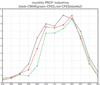
4. Some results of a coupled data assimilation experiment Using the improved CGCM, we have performed a 4D- VAR coupled data assimilation experiment, in which opti- mum values of the bulk parameters for air-sea fluxes (chosen as the control variables together with the initial condition) are sought by assimilating all the observational data available (e.g., PREPBUFFER for the atmosphere, and Reynolds SST, World Ocean Database1998, FNMOC, and TOPEX/POSEI- DON sea surface height anomaly data for the ocean). Our output exhibits significant improvement in the quantitative representation of seasonal change. For example, the annual march of global precipitation reflects most of observational features reported so far. In particular, the onset sequence of Indian monsoon rainfall is well reproduced (Fig. 7). Furthermore, In Figs. 8 and 9, the annual march of both the BAIU front and the storm track over the North Pacific is in good agreement with observations. In addtition, our sensitivi- ty experiment using the adjoint model clarified the probabili- ty density distribution of moisture sources of rainfall in sev- eral key regions (not shown), thereby enabling us to identify

298.5

298

297.5

297

296.5

296

295.5

295

294.5

294 JAN FEB MAR APR MAY JUN JUL AUG SEP OCT NOV DEC

SST (Peruvian)

Fig. 5 10-year averaged seasonal variations of SST [K] over the Peruvian region for CTL-C (solid), ANL-C (dotted), NoSC-C (broken) experiments and OISST observation (1991–2000) (dashed-dotted).

DEC NOV OCT SEP AUG JUL JUN MAY APR MAR FEB

JAN

140E 160E 180 160W 140W 120W 100W 80W 140E 160E 180 160W 140W 120W 100W 80W 140E 160E 180 160W 140W 120W 100W 80W 140E 160E 180 160W 140W 120W 100W 80W

(a) NoSC–C (b) ANL–C (c) CTL–C (d) OISST

Fig. 6 10-year averaged monthly SST fluctuations from the annual averaged values in each grid point for (a) NoSC-C, (b) ANL-C, (c) CT-C experiments and (d) OISST observation averaged over 2°S–2°N. The dark shaded regions denote areas greater than 0.5 degC and the light shaded regions those less than –0.5 degC.

the major source regions. These results suggest that our improved data assimilation system is capable of representing the dynamical state of the global environment than earlier models and further creating new information for better under- standing of climate change mechanisms.

5. Concluding remarks

A diagnostic scheme for marine stratocumulus cloud cover has been developed using a GCM approach. As a result, the SCu cloud cover simulated by the new scheme can display more realistic spatial distributions. The vertical structures of SCu and the related atmospheric variables of the lower tropo- sphere, such as temperature, moisture and heating rate, are considerably improved in the Peruvian region where strong SCu is observed. When the new scheme is applied within a coupled GCM, improved downward shortwave radiation fluxes at the sea surface resulting from the realistically simu-

10

9

8

7

6

5

4

3

2

1

0JAN

1979 ^{FEB MAR APR MAY JUN JUL AUG SEP OCT NOV DEC}

monthly PRCP: Indochina black–CMAP,green–CFES,red–CFESda(e4s2)

Fig. 7 Annual march of precipitation in the Indo-China Peninsula. Black: Observation (CMAP). Red: Assimilation. Green: Simulation. (horizontal axis: month; vertical axis: precipitation)

50N 45N 40N 35N 30N 25N 20N 15N 10N 5N EQ

50N 45N 40N 35N 30N 25N 20N 15N 10N 5N

JAN FEB MAR APR MAY JUN JUL AUG SEP OCT NOV DEC EQJAN FEB MAR APR MAY JUN JUL AUG SEP OCT NOV DEC

prcp 4d7ens4s2 (130E–145E) prcp jun (130E–145E)

2 4 6 8 10 12 14 16 18

2 4 6 8 10 12 14 16 18

K7CFES (160E–180) K7CFESdo (160E–180) CMAP (160E–180)

K7CFES (170W–150W) K7CFESdo (170W–150W) CMAP (170W–150W) Fig. 8 Time-space cross section of daily mean precipitation in the region of 0–50N and

160–180E. Left: Assimilation. Right: Observation (GPCP).

Fig. 9 Annual march of precipitation in the North Pacific region. Left: Simulation. Middle: Assimilation. Right: Observation (CMAP).

lated SCu cause the SST west of the continents in the sub- tropics to display weakened warm biases and more realistic seasonal cycles. The new scheme makes not only a local modification but also large-scale modifications to the model climatology in the low-latitudes of the eastern Pacific. A shallow meridional circulation across the equator is excited, and the strength and location of ITCZ and the seasonal cycle of equatorial SST are also improved. These large-scale improvements are consistent with the results of previous sen- sitivity studies in which the observational cloudiness is exter- nally given. The results of sensitivity experiments of slow upward transport suggest that estimations by 4D-VAR data assimilation techniques could be useful in the control of sim- ple parameters for low level clouds and moisture in improved model climatologies. Since it is not easy to estimate the strength of such slow and weak vertical motion associated with the SCu from observations, a 4D-VAR data assimilation method (best model parameter estimation) based on control of the vertical coefficients is a useful method of improving the vertical structures of moisture. Indeed, our assimilation result illustrates the superiority of our 4D-VAR coupled data assimilation system and therefore underline its usefulness for understanding the nature of climate variability and in formu- lating accurate forecasts.

References

Arakawa, A., and W. H. Schubert, Interaction of cumulus cloud ensemble with the large–scale environment. Part I, J. Atmos. Sci., 31, 674–701, 1974.

Bachiochi, D. R., and T. N. Krishnamurti, Enhanced low- level stratus in the FSU coupled ocean-atmosphere model, Mon. Wea. Rev., 128, 3083–3013, 2000. Bretherton, C. S., J. R. McCaa, and H. Grenier, A new para-

meterization for shallow cumulus convection and its application to marine subtropical cloud–topped bound- ary layers. Part I: Description and 1D results, Mon. Wea. Rev., 132, 864–882, 2004.

Dai, A., Precipitation characteristics in eighteen coupled cli- mate models, J. Climate, submitted, 2005b.

Gordon, C. T., A. Rosati, and R. Gudgel (2000), Tropical sensitivity of a coupled model to specified ISCCP low clouds, J. Climate, 13, 2239–2260, 2000.

Hibler, W. D. III, Modeling a variable thickness sea ice cover, Mon. Wea. Rev., 1, 1943–1973, 1980.

Komori, N., K. Takahashi, K. Komine, T. Motoi, X. Zhang, and G. Sagawa, Description of sea-ice component of Coupled Ocean-Sea-Ice Model for the Earth Simulator (OIFES), J. Earth Simulator, 4, 31–45, 2005.

Mechoso, C. R. et al., The seasonal cycle over the tropical Pacific in general circulation models, Mon. Wea. Rev.,

123, 2825–2838, 1995.

Moorthi S., and M.J. Suarez, Relaxed Arakawa-Schubert. A parameterization of moist convection for general circu- lation models, Mon. Wea. Rev., 120, 978–1002, 1992. Nakajima T., M. Tsukamoto, Y. Tsushima, A. Numaguti,

and T. Kimura, Modeling of the radiative process in an atmospheric general circulation model, Appl. Opt., 39, 4869–4878, 2000.

Philander, S. G. H., D. Gu, G. Lambert, T. Li, D. Halpern, N.-C. Lau, and R. C. Pacanowski, Why the ITCZ is mostly north of the equator, J. Climate, 9, 2958–2972, 1996.

Ohfuchi, W., H. Nakamura, M. K. Yoshioka, T. Enomoto, K. Takaya, X. Peng, S. Yamane, T. Nishimura, Y. Kurihara, and K. Ninomiya, 10-km mech meso–scale resolving simulations of the global atmosphere on the Earth Simulator: Preliminary outcomes of AFES (AGCM for the Earth Simulator), J. Earth Simulator, 1, 8–34, 2004. Sekiguchi M., T. Nakajima, K. Suzuki, K. Kawamoto, A.

Higurashi, D. Rosenfeld, I. Sano, and S. Mukai, A study of the direct and indirect effects of aerosols using global satellite data sets of aerosol and cloud parameters, J. Geophys. Res., 108, 4699, doi10.1029/2002JD003359, 2003.

Slingo, J. M., The development and verification of a cloud prediction scheme for the ECMWF model, Q. J. R. Meteor. Soc., 113, 899–927, 1987.

Teixeira, J., and T. F. Hogan Boundary layer clouds in a global atmospheric model: simple cloud cover parame- terizations, J. Climate, 15, 1261–1276, 2002.

Wang, Y., S.-P. Xie, H. Xu, and B. Wang , Regional Model Simulations of Marine Boundary Layer Clouds over the Southeast Pacific off South America. Part I: Control Experiment, Mon. Wea. Rev., 132, 274–296, 2004a. Wang, Y., H. Xu, and S.-P. Xie (2004b), Regional Model

Simulations of Marine Boundary Layer Clouds over the Southeast Pacific off South America. Part II: Sensitivity Experiments, Mon. Wea. Rev., 132, 2650–2668, 2004b. Wang, Y., S.-P. Xie, B. Wang, and H. Xu (2005), Large-

scale atmospheric forcing by Southeast Pacific bound- ary layer clouds: A regional model study, J. Climate, 18, 934–951, 2005.

Xu, H., Y. Wang, and S.-P. Xie (2004), Effects of the Andes on Eastern Pacific climate: a regional atmospheric model study, J. Climate, 17, 589–602, 2005.

Yu, J.-Y., and C. R. Mechoso (1999), Links between annual variations of Peruvian stratocumulus clouds and of SST in the eastern equatorial Pacific, J. Climate, 12, 3305–3318, 1999.

1, 2 1 1 1 1 1 1

2 3 5 4 3

1 2 3

4 NEC

5

MAT-

SIRO IPRC

(1986 2004 19 ) 3 SST

0.78K 1.87K

Argo