(will be inserted by the editor)
Variational Bayesian Sparse Additive Matrix
Factorization
Shinichi Nakajima · Masashi Sugiyama · S. Derin Babacan
Received: date / Accepted: date
Abstract Principal component analysis (PCA) approximates a data matrix with a low-rank one by imposing sparsity on its singular values. Its robust variant can cope with spiky noise by introducing an element-wise sparse term. In this paper, we extend such sparse matrix learning methods, and propose a novel framework called sparse additive matrix factorization (SAMF). SAMF systematically induces various types of sparsity by a Bayesian regularization effect, called model-induced regularization. Although group LASSO also allows us to design arbitrary types of sparsity on a matrix, SAMF, which is based on the Bayesian framework, pro- vides inference without any requirement for manual parameter tuning. We propose an efficient iterative algorithm called the mean update (MU) for the variational Bayesian approximation to SAMF, which gives the global optimal solution for a large subset of parameters in each step. We demonstrate the usefulness of our method on benchmark datasets and a foreground/background video separation problem.
Keywords variational Bayes · robust PCA · matrix factorization · sparsity · model-induced regularization
Shinichi Nakajima
Nikon Corporation, 1-6-3 Nishi-ohi, Shinagawa-ku, Tokyo 140-8601, Japan Tel.: +81-3-3773-1517
Fax: +81-3-3775-5934
E-mail: [email protected] Masashi Sugiyama
Department of Computer Science, Tokyo Institute of Technology, 2-12-1-W8-74 O-okayama, Meguro-ku, Tokyo 152-8552, Japan
E-mail: [email protected] S. Derin Babacan
Google Inc., 1900 Charleston Rd, Mountain View, CA 94043 USA E-mail: [email protected]
1 Introduction
Principal component analysis (PCA) (Hotelling, 1933) is a classical method for obtaining low-dimensional expression of data. PCA can be regarded as approxi- mating a data matrix with a low-rank one by imposing sparsity on its singular values. A robust variant of PCA further copes with sparse spiky noise included in observations (Cand`es et al., 2011; Ding et al., 2011; Babacan et al., 2012).
In this paper, we extend the idea of robust PCA, and propose a more gen- eral framework called sparse additive matrix factorization (SAMF). The proposed SAMF can handle various types of sparse noise such as row-wise and column-wise sparsity, in addition to element-wise sparsity (spiky noise) and low-rank sparsity (low-dimensional expression); furthermore, their arbitrary additive combination is also allowed. In the context of robust PCA, row-wise and column-wise sparsity can capture noise observed when some sensors are broken and their outputs are always unreliable, or some accident disturbs all sensor outputs at a time.
Flexibility of SAMF in sparsity design allows us to incorporate side information more efficiently. We show such an example in foreground/background video sep- aration, where sparsity is induced based on image segmentation. Although group LASSO (Yuan and Lin, 2006; Raman et al., 2009) also allows arbitrary sparsity de- sign on matrix entries, SAMF, which is based on the Bayesian framework, enables us to estimate all unknowns from observations, and allows us to enjoy inference without manual parameter tuning.
Technically, our approach induces sparsity by the so-called model-induced reg- ularization (MIR) (Nakajima and Sugiyama, 2011). MIR is an implicit regular- ization property of the Bayesian approach, which is based on one-to-many (i.e., redundant) mapping of parameters and outcomes (Watanabe, 2009). In the case of matrix factorization, an observed matrix is decomposed into two redundant matrices, which was shown to induce sparsity in the singular values under the variational Bayesian approximation (Nakajima and Sugiyama, 2011).
We show that MIR in SAMF can be interpreted as automatic relevance deter- mination (ARD) (Neal, 1996), which is a popular Bayesian approach to inducing sparsity. Nevertheless, we argue that the MIR formulation is more preferable since it allows us to derive a practically useful algorithm called the mean update (MU) from a recent theoretical result (Nakajima et al., 2013): The MU algorithm is based on the variational Bayesian approximation, and gives the global optimal so- lution for a large subset of parameters in each step. Through experiments, we show that the MU algorithm compares favorably with a standard iterative algorithm for variational Bayesian inference.
2 Formulation
In this section, we formulate the sparse additive matrix factorization (SAMF) model.
2.1 Examples of Factorization
In standard MF, an observed matrix V ∈ RL×M is modeled by a low rank target matrix U ∈ RL×M contaminated with a random noise matrixE ∈ RL×M.
V = U +E.
Then the target matrix U is decomposed into the product of two matrices A ∈ RM ×H and B∈ RL×H:
Ulow-rank= BA⊤=
∑H h=1
bha⊤h, (1)
where ⊤ denotes the transpose of a matrix or vector. Throughout the paper, we denote a column vector of a matrix by a bold small letter, and a row vector by a bold small letter with a tilde:
A = (a1, . . . , aH) = (ea1, . . . ,aeM)⊤, B = (b1, . . . , bH) = (eb1, . . . , ebL)⊤.
The last equation in Eq.(1) implies that the plain matrix product (i.e., BA⊤) is the sum of rank-1 components. It was elucidated that this product induces an implicit regularization effect called model-induced regularization (MIR), and a low- rank (singular-component-wise sparse) solution is produced under the variational Bayesian approximation (Nakajima and Sugiyama, 2011).
Let us consider other types of factorization:
Urow= ΓED = (γ1eed1, . . . , γLedeL)⊤, (2) Ucolumn= EΓD= (γ1de1, . . . , γMd eM), (3) where ΓD = diag(γ1d, . . . , γdM)∈ RM ×M and ΓE = diag(γe1, . . . , γLe)∈ RL×L are diagonal matrices, and D, E ∈ RL×M. These examples are also matrix products, but one of the factors is restricted to be diagonal. Because of this diagonal con- straint, the l-th diagonal entry γle in ΓE is shared by all the entries in the l-th row of Urow as a common factor. Similarly, the m-th diagonal entry γmd in ΓD is shared by all the entries in the m-th column of Ucolumn.
Another example is the Hadamard (or element-wise) product:
Uelement= E∗ D, where (E ∗ D)l,m= El,mDl,m. (4) In this factorization form, no entry in E and D is shared by more than one entry in Uelement.
In fact, the forms (2)–(4) of factorization induce different types of sparsity, through the MIR mechanism. In Section 2.2, they will be derived as a row-wise, a column-wise, and an element-wise sparsity inducing terms, respectively, within a unified framework.
!→
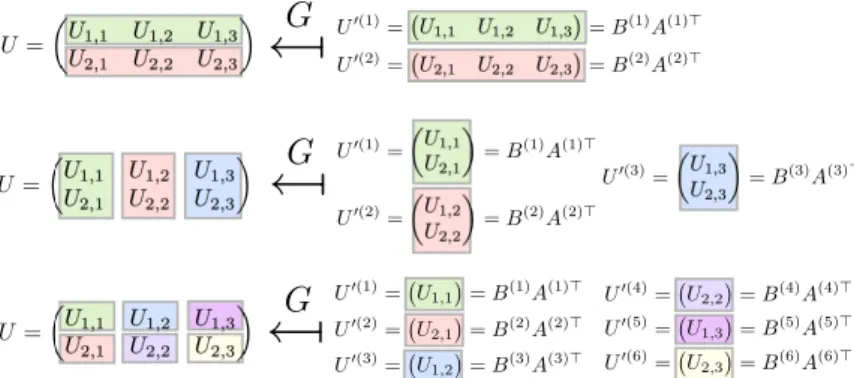
Fig. 1 An example of SMF-term construction. G(·; X ) with X : (k, l′, m′) 7→ (l, m) maps the set {U′(k)}Kk=1 of the PR matrices to the target matrix U , so that Ul′(k)′,m′= UX(k,l′,m′)= Ul,m.
!→
G
U =!UU1,1 U1,2 U1,3
2,1 U2,2 U2,3
" U′(1)
=!U1,1 U1,2 U1,3"= B(1)A(1)⊤ U′(2)=!U2,1 U2,2 U2,3"= B(2)A(2)⊤
!→
G
U =!UU1,1 U1,2 U1,3
2,1 U2,2 U2,3
" U
′(1)=
!U1,1 U2,1
"
= B(1)A(1)⊤
U′(2)=!U1,2 U2,2
"
= B(2)A(2)⊤ U′(3)
=
!U1,3 U2,3
"
= B(3)A(3)⊤
!→
G
U =!UU1,1 U1,2 U1,3
2,1 U2,2 U2,3
"
U′(1)=!U1,1"= B(1)A(1)⊤
U′(6)=!U2,3"= B(6)A(6)⊤ U′(2)=!U2,1"= B(2)A(2)⊤
U′(3)=!U1,2"= B(3)A(3)⊤
U′(4)=!U2,2"= B(4)A(4)⊤ U′(5)=!U1,3"= B(5)A(5)⊤
Fig. 2 SMF-term construction for the row-wise (top), the column-wise (middle), and the element-wise (bottom) sparse terms.
2.2 A General Expression of Factorization
Our general expression consists of partitioning, rearrangement, and factorization. The following is the form of a sparse matrix factorization (SMF) term:
U = G({U′(k)}Kk=1;X ), where U′(k)= B(k)A(k)⊤. (5) Here, {A(k), B(k)}Kk=1 are parameters to be estimated, and G(·; X ) : R∏Kk=1(L′(k)×M′(k))7→ RL×M is a designed function associated with an index map- ping parameterX , which will be explained shortly.
Figure 1 shows how to construct an SMF term. First, we partition the en- tries of U into K parts. Then, by rearranging the entries in each part, we form partitioned-and-rearranged (PR) matrices U′(k) ∈ RL′(k)×M′(k) for k = 1, . . . , K. Finally, each of U′(k) is decomposed into the product of A(k)∈ RM′(k)×H′(k) and B(k)∈ RL′(k)×H′(k), where H′(k) ≤ min(L′(k), M′(k)).
In Eq.(5), the function G(·; X ) is responsible for partitioning and rearrange- ment: It maps the set {U′(k)}Kk=1 of the PR matrices to the target matrix U ∈ RL×M, based on the one-to-one map X : (k, l′, m′) 7→ (l, m) from the in- dices of the entries in{U′(k)}Kk=1 to the indices of the entries in U , such that
(G({U′(k)}Kk=1;X ))
l,m= Ul,m= UX(k,l
′,m′)= Ul′(k)′,m′. (6)
Table 1 Examples of SMF term. See the main text for details.
Factorization Induced sparsity K (L′(k), M′(k)) X : (k, l′, m′) 7→ (l, m) U = BA⊤ low-rank 1 (L, M ) X (1, l′, m′) = (l′, m′) U = ΓED row-wise L (1, M ) X (k, 1, m′) = (k, m′) U = EΓD column-wise M (L, 1) X (k, l′, 1) = (l′, k) U = E ∗ D element-wise L × M (1, 1) X (k, 1, 1) = vec-order(k)
As will be discussed in Section 4.1, the SMF-term expression (5) under the variational Bayesian approximation induces low-rank sparsity in each partition. This means that partition-wise sparsity is also induced. Accordingly, partition- ing, rearrangement, and factorization should be designed in the following manner. Suppose that we are given a required sparsity structure on a matrix (examples of possible side information that suggests particular sparsity structures are given in Section 2.3). We first partition the matrix, according to the required sparsity. Some partitions can be submatrices. We rearrange each of the submatrices on which we do not want to impose low-rank sparsity into a long vector (U′(3) in the example in Figure 1). We leave the other submatrices which we want to be low-rank (U′(2)), the vectors (U′(1)and U′(4)) and the scalars (U′(5)) as they are. Finally, we factorize each of the PR matrices to induce sparsity through the MIR mechanism.
Let us, for example, assume that row-wise sparsity is required. We first make the row-wise partition, i.e., separate U ∈ RL×M into L pieces of M -dimensional row vectors U′(l) = ue⊤l ∈ R1×M. Then, we factorize each partition as U′(l) = B(l)A(l)⊤(see the top illustration in Figure 2). Thus, we obtain the row-wise sparse term (2). Here, X (k, 1, m′) = (k, m′) makes the following connection between Eqs.(2) and (5): γle= B(k)∈ R, edl= A(k)∈ RM ×1 for k = l. Similarly, requiring column-wise and element-wise sparsity leads to Eqs.(3) and (4), respectively (see the bottom two illustrations in Figure 2). Table 1 summarizes how to design these SMF terms, where vec-order(k) = (1 + ((k− 1) mod L), ⌈k/L⌉) goes along the columns one after another in the same way as the vec operator forming a vector by stacking the columns of a matrix (in other words, (U′(1), . . . , U′(K))⊤= vec(U )).
2.3 Sparse Additive Matrix Factorization
We define a sparse additive matrix factorization (SAMF) model as the sum of SMF terms (5):
V =
∑S s=1
U(s)+E, (7)
where U(s)= G({B(k,s)A(k,s)⊤}Kk=1(s);X(s)). (8) In practice, SMF terms should be designed based on side information. Suppose that V ∈ RL×Mconsists of M samples of L-dimensional sensor outputs. In robust PCA (Cand`es et al., 2011; Ding et al., 2011; Babacan et al., 2012), an element- wise sparse term is added to the low-rank term, which is expected to be the clean signal, when sensor outputs are expected to contain spiky noise:
V = Ulow-rank+ Uelement+E. (9)
background foreground Fig. 3 Foreground/background video separation task.
time
pixels
V
Fig. 4 The observation matrix V is constructed by stacking all pixels in each frame into each column.
time pixels
pre-segmentation
Fig. 5 Construction of a segment-wise sparse term. The original frame is pre-segmented and the sparseness is induced in a segment-wise manner. Details are described in Section 5.4.
Here, it can be said that the “expectation of spiky noise” is used as side informa- tion.
Similarly, if we suspect that some sensors are broken, and their outputs are unreliable over all M samples, we should prepare the row-wise sparse term to capture the expected row-wise noise, and try to keep the estimated clean signal Ulow-rank uncontaminated with the row-wise noise:
V = Ulow-rank+ Urow+E.
If we know that some accidental disturbances occurred during the observation, but do not know their exact locations (i.e., which samples are affected), the column- wise sparse term can effectively capture these disturbances.
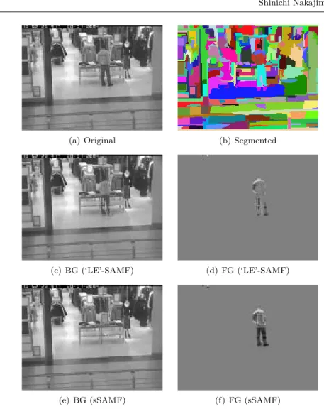
The SMF expression (5) enables us to use side information in a more flex- ible way. In Section 5.4, we show that our method can be applied to a fore- ground/background video separation problem, where moving objects (such as a person in Figure 3) are considered to belong to the foreground. Previous ap- proaches (Cand`es et al., 2011; Ding et al., 2011; Babacan et al., 2012) constructed the observation matrix V by stacking all pixels in each frame into each column (Figure 4), and fitted it by the model (9). Here, the low-rank term and the element- wise sparse term are expected to capture the static background and the moving foreground, respectively. However, we can also rely on a natural assumption that a pixel segment having similar intensity values in an image tends to belong to the same object. Based on this side information, we adopt a segment-wise sparse term, where the PR matrix is constructed using a precomputed over-segmented image (Figure 5). We will show in Section 5.4 that the segment-wise sparse term captures the foreground more accurately than the element-wise sparse term.
Let us summarize the parameters of the SAMF model (7) as follows:
Θ ={ΘA(s), ΘB(s)}Ss=1, where Θ(s)A ={A(k,s)}Kk=1(s), Θ(s)B ={B(k,s)}Kk=1(s). As in the probabilistic MF (Salakhutdinov and Mnih, 2008), we assume indepen- dent Gaussian noise and priors. Thus, the likelihood and the priors are written as
p(V|Θ) ∝ exp
−2σ12 V −
∑S s=1
U(s)
2
Fro
, (10)
p({Θ(s)A }Ss=1)∝ exp (
−12
∑S s=1
K∑(s) k=1
tr(A(k,s)CA(k,s)−1A(k,s)⊤) )
, (11)
p({Θ(s)B }Ss=1)∝ exp (
−12
∑S s=1
K∑(s) k=1
tr(B(k,s)CB(k,s)−1B(k,s)⊤) )
, (12)
where ∥ · ∥Fro and tr(·) denote the Frobenius norm and the trace of a matrix, respectively. We assume that the prior covariances of A(k,s)and B(k,s)are diagonal and positive-definite:
CA(k,s)= diag(c(k,s)2a1 , . . . , c(k,s)2aH ), CB(k,s)= diag(c(k,s)2b1 , . . . , c(k,s)2bH ).
Without loss of generality, we assume that the diagonal entries of CA(k,s)CB(k,s)are arranged in the non-increasing order, i.e., c(k,s)ah c(k,s)b
h ≥ c(k,s)ah′ c (k,s)
bh′ for any pair h < h′.
2.4 Variational Bayesian Approximation The Bayes posterior is written as
p(Θ|V ) = p(V|Θ)p(Θ)
p(V ) , (13)
where p(V ) = ⟨p(V |Θ)⟩p(Θ) is the marginal likelihood. Here, ⟨·⟩p denotes the expectation over the distribution p. Since the Bayes posterior (13) for matrix fac- torization is computationally intractable, the variational Bayesian (VB) approx- imation was proposed (Bishop, 1999; Lim and Teh, 2007; Ilin and Raiko, 2010; Babacan et al., 2012).
Let r(Θ), or r for short, be a trial distribution. The following functional with respect to r is called the free energy:
F (r|V ) =
⟨
log r(Θ) p(V|Θ)p(Θ)
⟩
r(Θ)
=
⟨
log r(Θ) p(Θ|V )
⟩
r(Θ)
− log p(V ). (14)
The first term is the Kullback-Leibler (KL) distance from the trial distribution to the Bayes posterior, and the second term is a constant. Therefore, minimizing the free energy (14) amounts to finding a distribution closest to the Bayes posterior in the sense of the KL distance. In the VB approximation, the free energy (14) is minimized over some restricted function space.
Following the standard VB procedure (Bishop, 1999; Lim and Teh, 2007; Baba- can et al., 2012), we impose the following decomposability constraint on the pos- terior:
r(Θ) =
∏S s=1
rA(s)(ΘA(s))rB(s)(Θ(s)B ). (15)
Under this constraint, it is easy to show that the VB posterior minimizing the free energy (14) is written as
r(Θ) =
∏S s=1
K∏(s) k=1
(M′(k,s)
∏
m′=1
NH′(k,s)(ae(k,s)m′ ; eba(k,s)m′ , ΣA(k,s))
·
L∏′(k,s) l′=1
NH′(k,s)(eb (k,s) l′ ; ebb
(k,s) l′ , ΣB(k,s))
)
, (16)
where Nd(·; µ, Σ) denotes the d-dimensional Gaussian distribution with mean µ and covariance Σ.
3 Algorithm for SAMF
In this section, we first present a theorem that reduces a partial SAMF problem to the standard MF problem, which can be solved analytically. Then we derive an algorithm for the entire SAMF problem.
3.1 Key Theorem
Let us denote the mean of U(s), defined in Eq.(8), over the VB posterior by Ub(s)=⟨U(s)⟩r(s)
A (Θ (s) A )r
(s) B (Θ
(s) B )
= G({ bB(k,s)Ab(k,s)⊤}Kk=1(s);X(s)). (17) Then we obtain the following theorem (its proof is given in Appendix A): Theorem 1 Given { bU(s′)}s′̸=s and the noise variance σ2, the VB posterior of (Θ(s)A , Θ(s)B ) ={A(k,s), B(k,s)}Kk=1(s) coincides with the VB posterior of the following MF model:
p(Z′(k,s)|A(k,s), B(k,s))∝exp (
−2σ12 Z′(k,s)− B(k,s)A(k,s)⊤ 2Fro )
, (18) p(A(k,s))∝exp
(
−12tr(A(k,s)CA(k,s)−1A
(k,s)⊤)), (19)
p(B(k,s))∝exp (
−12tr(B(k,s)CB(k,s)−1B
(k,s)⊤)), (20)
for each k = 1, . . . , K(s). Here, Z′(k,s)∈ RL′(k,s)×M′(k,s) is defined as Zl′(k,s)′,m′ = ZX(s)(s)(k,l′,m′), where Z
(s)= V
−∑
s′̸=s
Ub(s). (21)
The left formula in Eq.(21) relates the entries of Z(s) ∈ RL×M to the entries of {Z′(k,s) ∈ RL′(k,s)×M′(k,s)}k=1K(s) by using the map X(s) : (k, l′, m′) 7→ (l, m) (see Eq.(6) and Figure 1).
Theorem 1 states that a partial problem of SAMF—finding the posterior of (A(k,s), B(k,s)) for each k = 1, . . . , K(s), given{ bU(s′)}s′̸=sand σ2— can be solved in the same way as in the standard VBMF, to which the global analytic solution is available (Nakajima et al., 2013). Based on this theorem, we will propose a useful algorithm in the following subsections.
The noise variance σ2 is also unknown in many applications. To estimate σ2, we can use the following lemma (its proof is also included in Appendix A): Lemma 1 Given the VB posterior for{Θ(s)A , Θ(s)B }Ss=1, the noise variance σ2min- imizing the free energy (14) is given by
σ2= 1 LM
{
∥V ∥2Fro− 2
∑S s=1
tr (
Ub(s)⊤ (
V−
∑S s′=s+1
Ub(s′) ))
+
∑S s=1
K∑(s) k=1
tr(( bA(k,s)⊤Ab(k,s)+ M′(k,s)ΣA(k,s))
· ( bB(k,s)⊤Bb(k,s)+ L′(k,s)ΣB(k,s))
)}
. (22)
3.2 Partial Analytic Solution
Theorem 1 allows us to use the results given in Nakajima et al. (2013), which provide the global analytic solution for VBMF. Although the free energy of VBMF is also non-convex, Nakajima et al. (2013) showed that the minimizers can be written as a reweighted singular value decomposition. This allows one to solve the minimization problem separately for each singular component, which facilitated the analysis. By finding all stationary points and calculating the free energy on them, they successfully obtained an analytic-form of the global VBMF solution.
Combining Theorem 1 above and Theorems 3–5 in Nakajima et al. (2013), we obtain the following corollaries:
Corollary 1 Assume that L′(k,s) ≤ M′(k,s) for all (k, s), and that { bU(s′)}s′̸=s
and the noise variance σ2 are given. Let γh(k,s) (≥ 0) be the h-th largest singular value of Z′(k,s), and let ω(k,s)ah and ω(k,s)bh be the associated right and left singular vectors:
Z′(k,s)=
L∑′(k,s) h=1
γh(k,s)ω(k,s)b
h ω
(k,s)⊤
ah . (23)
Let bγ(k,s)second
h be the second largest real solution of the following quartic equation with respect to t:
fh(t) := t4+ ξ3(k,s)t3+ ξ2(k,s)t2+ ξ1(k,s)t + ξ0(k,s)= 0, (24) where the coefficients are defined by
ξ3(k,s)= (L
′(k,s)− M′(k,s))2γ(k,s) h
L′(k,s)M′(k,s) , ξ2(k,s)=−
(
ξ3γh(k,s)+(L
′(k,s)2+ M′(k,s)2)η(k,s)2 h
L′(k,s)M′(k,s) +
2σ4 c(k,s)2ah c(k,s)2b
h
) ,
ξ1(k,s)= ξ(k,s)3
√ ξ0(k,s), ξ0(k,s)=
(
η(k,s)2h − σ
4
c(k,s)2ah c(k,s)2bh )2
,
ηh(k,s)2= (
1−σ
2L′(k,s)
γh(k,s)2 ) (
1− σ
2M′(k,s)
γ(k,s)2h )
γh(k,s)2.
Let
eγh(k,s)=
√
τ +√τ2− L′(k,s)M′(k,s)σ4, (25) where
τ = (L
′(k,s)+ M′(k,s))σ2
2 +
σ4 2c(k,s)2ah c(k,s)2bh .
Then, the global VB solution can be expressed as Ub′(k,s)VB= ( bB(k,s)Ab(k,s)⊤)VB=
H∑′(k,s) h=1
bγh(k,s)VBω(k,s)bh ω(k,s)⊤ah ,
where bγh(k,s)VB=
{bγ(k,s)second
h if γ
(k,s) h > eγ
(k,s)
h ,
0 otherwise. (26)
Corollary 2 Assume that L′(k,s)≤ M′(k,s) for all (k, s). Given{ bU(s′)}s′̸=s and the noise variance σ2, the global empirical VB solution (where the hyperparam- eters {CA(k,s), CB(k,s)} are also estimated from observation) is given by
Ub′(k,s)EVB=
H∑′(k,s) h=1
bγh(k,s)EVBω (k,s) bh ω
(k,s)⊤ ah ,
where bγh(k,s)EVB=
{γ˘(k,s)VBh if γh(k,s)> γ(k,s)h and ∆(k,s)h ≤ 0,
0 otherwise. (27)
Here, γ(k,s)
h = (
√L′(k,s)+√M′(k,s))σ, (28)
˘
c(k,s)2h = 1 2L′(k,s)M′(k,s)
(
γh(k,s)2− (L′(k,s)+ M′(k,s))σ2
+√(γh(k,s)2− (L′(k,s)+ M′(k,s))σ2)2− 4L′(k,s)M′(k,s)σ4 )
, (29)
∆(k,s)h = M′(k,s)log
( γh(k,s) M′(k,s)σ2˘γ
(k,s)VB
h + 1
)
+ L′(k,s)log
( γh(k,s) L′(k,s)σ2˘γ
(k,s)VB
h + 1
)
+ 1 σ2
(−2γh(k,s)˘γ (k,s)VB
h + L
′(k,s)
M′(k,s)c˘(k,s)2h ), (30) and ˘γh(k,s)VB is the VB solution for c(k,s)ah c(k,s)bh = ˘c(k,s)h .
Corollary 3 Assume that L′(k,s)≤ M′(k,s) for all (k, s). Given{ bU(s′)}s′̸=s and the noise variance σ2, the VB posteriors are given by
rAVB(k,s)(A(k,s)) =
H∏′(k,s) h=1
NM′(k,s)(a(k,s)h ;ba(k,s)h , σ (k,s)2
ah IM′(k,s)),
rVBB(k,s)(B(k,s)) =
H∏′(k,s) h=1
NL′(k,s)(b(k,s)h ; bb (k,s)
h , σ(k,s)2bh IL′(k,s)),
where, for bγh(k,s)VB being the solution given by Corollary 1, b
a(k,s)h =±
√
bγ(k,s)VBh δb (k,s)
h · ω(k,s)ah , bb (k,s)
h =±
√
bγh(k,s)VBbδ (k,s)−1
h · ω(k,s)bh ,
σ(k,s)2ah = 1
2M′(k,s)(bγ(k,s)VBh bδh(k,s)−1+ σ2c(k,s)−2ah )
· {
−(bη(k,s)2h − σ2(M′(k,s)− L′(k,s)))
+
√
(bη(k,s)2h − σ2(M′(k,s)− L′(k,s)))2+ 4M′(k,s)σ2ηbh(k,s)2
} ,
σ(k,s)2bh = 1
2L′(k,s)(bγh(k,s)VBbδh(k,s)+ σ2c(k,s)−2b
h )
· {
−(bη(k,s)2h + σ
2(M′(k,s)− L′(k,s)))
+
√
(bη(k,s)2h + σ2(M′(k,s)− L′(k,s)))2+ 4L′(k,s)σ2ηb(k,s)2h
} ,
δb(k,s)h = 1
2σ2M′(k,s)c(k,s)−2ah
{
(M′(k,s)− L′(k,s))(γ(k,s)h − bγh(k,s)VB)
+
√
(M′(k,s)− L′(k,s))2(γh(k,s)− bγh(k,s)VB)2+ 4σ4L′(k,s)M′(k,s) c(k,s)2ah c(k,s)2bh
} ,
b η(k,s)2h =
ηh(k,s)2 if γh(k,s)> eγh(k,s),
σ4
c(k,s)2ah c(k,s)2bh otherwise.
Note that the corollaries above assume that L′(k,s) ≤ M′(k,s) for all (k, s). How- ever, we can easily obtain the result for the case when L′(k,s)> M′(k,s)by consid- ering the transpose bU′(k,s)⊤of the solution. Also, we can always take the mapping X(s) so that L′(k,s)≤ M′(k,s)holds for all (k, s) without any practical restriction. This eases the implementation of the algorithm.
When σ2 is known, Corollary 1 and Corollary 2 provide the global analytic solution of the partial problem, where the variables on which{ bU(s′)}s′̸=sdepends are fixed. Note that they give the global analytic solution for single-term (S = 1) SAMF.
3.3 Mean Update Algorithm
Using Corollaries 1–3 and Lemma 1, we propose an algorithm for SAMF, which we call the mean update (MU) algorithm. We describe its pseudo-code in Algo- rithm 1, where 0(d1,d2) denotes the d1× d2 matrix with all entries equal to zero. Note that, under the empirical Bayesian framework, all unknown parameters are estimated from observation, which allows inference without manual parameter tuning.
The MU algorithm is similar in spirit to the backfitting algorithm (Hastie and Tibshirani, 1986; D’Souza et al., 2004), where each additive term is updated to fit a dummy target. In the MU algorithm, Z(s)defined in Eq.(21) corresponds to the dummy target in the backfitting algorithm. Although each of the corollaries and
Algorithm 1Mean update (MU) algorithm for (empirical) VB SAMF.
1: Initialization: bU(s)← 0(L,M )for s = 1, . . . , S, σ2← ∥V ∥2Fro/(LM ). 2: for s = 1 to S do
3: The (empirical) VB solution of U′(k,s)= B(k,s)A(k,s)⊤for each k = 1, . . . , K(s), given { bU(s′)}s′̸=s, is computed by Corollary 1 (Corollary 2).
4: Ub(s)← G({ bB(k,s)Ab(k,s)⊤}Kk=1(s); X(s)). 5: end for
6: σ2 is estimated by Lemma 1, given the VB posterior on {Θ(s)A , Θ(s)B }Ss=1 (computed by Corollary 3).
7: Repeat 2 to 6 until convergence.
the lemma above guarantee the global optimality for each step, the MU algorithm does not generally guarantee the simultaneous global optimality over the entire parameter space. Nevertheless, experimental results in Section 5 show that the MU algorithm performs very well in practice.
When Corollary 1 or Corollary 2 is applied in Step 3 of Algorithm 1, a singu- lar value decomposition (23) of Z′(k,s), defined in Eq.(21), is required. However, for many practical SMF terms, including the row-wise, the column-wise, and the element-wise terms as well as the segment-wise term (which will be defined in Section 5.4), Z′(k,s) ∈ RL′(k,s)×M′(k,s) is a vector or scalar, i.e., L′(k,s) = 1 or M′(k,s) = 1. In such cases, the singular value and the singular vectors are given simply by
γ1(k.s)=∥Z′(k,s)∥, ω(k.s)a1 = Z′(k,s)/∥Z′(k,s)∥, ω(k.s)b1 = 1 if L′(k,s)= 1, γ1(k.s)=∥Z′(k,s)∥, ω(k.s)a1 = 1, ω
(k.s) b1 = Z
′(k,s)
/∥Z′(k,s)∥ if M′(k,s)= 1.
4 Discussion
In this section, we first relate MIR to ARD. Then, we introduce the standard VB iteration for SAMF, which is used as a baseline in the experiments. After that, we discuss related previous work, and the limitation of the current work.
4.1 Relation between MIR and ARD
The MIR effect (Nakajima and Sugiyama, 2011) induced by factorization actu- ally has a close connection to the automatic relevance determination (ARD) effect (Neal, 1996). Assume CA= IH, where Id denotes the d-dimensional identity ma- trix, in the plain MF model (18)–(20) (here we omit the suffixes k and s for brevity), and consider the following transformation: BA⊤ 7→ U ∈ RL×M. Then, the likelihood (18) and the prior (19) on A are rewritten as
p(Z′|U) ∝ exp (
− 1 2σ2∥Z
′− U∥2Fro
)
, (31)
p(U|B) ∝ exp (
−12tr(U⊤(BB⊤)†U)), (32)
where† denotes the Moore-Penrose generalized inverse of a matrix. The prior (20) on B is kept unchanged. p(U|B) in Eq.(32) is so-called the ARD prior with the covariance hyperparameter BB⊤∈ RL×L. It is known that this induces the ARD effect, i.e., the empirical Bayesian procedure where the prior covariance hyperpa- rameter BB⊤is also estimated from observation induces strong regularization and sparsity (Neal, 1996); see also Efron and Morris (1973) for a simple Gaussian case. In the current context, Eq.(32) induces low-rank sparsity on U if no restriction on BB⊤is imposed. Similarly, we can show that (γle)2in Eq.(2), (γmd)2 in Eq.(3), and El,m2 in Eq.(4) act as prior variances shared by the entries in uel ∈ RM, um ∈ RL, and Ul,m ∈ R, respectively. This explains the mechanism how the factorization forms in Eqs.(2)–(4) induce row-wise, column-wise, and element-wise sparsity, respectively.
When we employ the SMF-term expression (5), MIR occurs in each partition. Therefore, partition-wise sparsity and low-rank sparsity in each partition is ob- served. Corollaries 1 and 2 theoretically support this fact: Small singular values are discarded by thresholding in Eqs.(26) and (27).
4.2 Standard VB Iteration
Following the standard procedure for the VB approximation (Bishop, 1999; Lim and Teh, 2007; Babacan et al., 2012), we can derive the following algorithm, which we call the standard VB iteration:
Ab(k,s)= σ−2Z′(k,s)⊤Bb(k,s)ΣA(k,s), (33) ΣA(k,s)= σ2(Bb(k,s)⊤Bb(k,s)+L′(k,s)ΣB(k,s)+σ2CA(k,s)−1)−1, (34) Bb(k,s)= σ−2Z′(k,s)Ab(k,s)ΣB(k,s), (35) ΣB(k,s)= σ2(Ab(k,s)⊤Ab(k,s)+M′(k,s)ΣA(k,s)+σ2CB(k,s)−1)−1. (36) Iterating Eqs.(33)–(36) for each (k, s) in turn until convergence gives a local min- imum of the free energy (14).
In the empirical Bayesian scenario, the hyperparameters {CA(k,s), C
(k,s)
B }Kk=1,(s)Ss=1 are also estimated from observations. The following update rules give a local minimum of the free energy:
c(k,s)2ah =∥ba(k,s)h ∥2/M′(k,s)+ (ΣA(k,s))hh, (37) c(k,s)2bh =∥bb(k,s)h ∥2/L′(k,s)+ (Σ(k,s)B )hh. (38)
When the noise variance σ2is unknown, it is estimated by Eq.(22) in each iteration. The standard VB iteration is computationally efficient since only a single parameter in { bA(k,s), ΣA(k,s), bB(k,s), ΣB(k,s), c(k,s)2ah , c(k,s)2bh }Kk=1,(s)Ss=1 is updated in each step. However, it is known that the standard VB iteration is prone to suffer from the local minima problem (Nakajima et al., 2013). On the other hand, although the MU algorithm also does not guarantee the global optimal- ity as a whole, it simultaneously gives the global optimal solution for the set
{ bA(k,s), ΣA(k,s), bB(k,s), Σ (k,s) B , c
(k,s)2 ah , c(k,s)2b
h }Kk=1(s) for each s in each step. In Sec- tion 5, we will experimentally show that the MU algorithm tends to give a better solution (i.e., with a smaller free energy) than the standard VB iteration.
4.3 Related Work
As widely known, traditional PCA is sensitive to outliers in data and generally fails in their presence. Robust PCA (Cand`es et al., 2011) was developed to cope with large outliers that are not modeled within the traditional PCA. Unlike methods based on robust statistics (Huber and Ronchetti, 2009; Fischler and Bolles, 1981; Torre and Black, 2003; Ke and Kanade, 2005; Gao, 2008; Luttinen et al., 2009; Lakshminarayanan et al., 2011), Cand`es et al. (2011) explicitly modeled the spiky noise with an additional element-wise sparse term (see Eq.(9)). This model can also be applied to applications where the task is to estimate the element-wise sparse term itself (as opposed to discarding it as noise). A typical such application is foreground/background video separation (Figure 3).
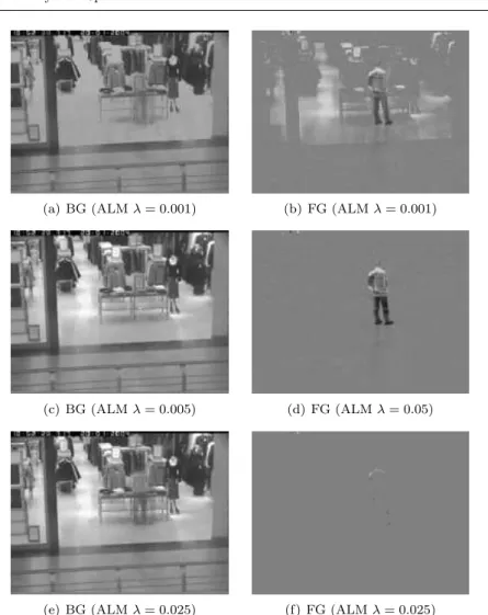
The original formulation of robust PCA is non-Bayesian, and the sparsity is induced by the ℓ1-norm regularization. Although its solution can be efficiently obtained via the augmented Lagrange multiplier (ALM) method (Lin et al., 2009), there are unknown algorithmic parameters that should be carefully tuned to obtain its best performance. Employing a Bayesian formulation addresses this issue: A sampling-based method (Ding et al., 2011) and a VB method (Babacan et al., 2012) were proposed, where all unknown parameters are estimated from the observation. Babacan et al. (2012) conducted an extensive experimental comparison be- tween their VB method, called a VB robust PCA, and other methods. They reported that the ALM method (Lin et al., 2009) requires careful tuning of its algorithmic parameters, and the Bayesian sampling method (Ding et al., 2011) has high computational complexity that can be prohibitive in large-scale applica- tions. Compared to these methods, the VB robust PCA is favorable both in terms of computational complexity and estimation performance.
Our SAMF framework contains the robust PCA model as a special case where the observed matrix is modeled as the sum of a low-rank and an element-wise sparse terms. The VB algorithm used in Babacan et al. (2012) is the same as the standard VB iteration introduced in Section 4.2, except a slight difference in the hyperprior setting. Accordingly, our proposal in this paper is an extension of the VB robust PCA in two ways—more variation in sparsity with different types of factorization and higher accuracy with the MU algorithm. In Section 5, we experimentally show advantages of these extensions. In our experiment, we use a SAMF counterpart of the VB robust PCA, named ‘LE’-SAMF in Section 5.1, with the standard VB iteration as a baseline method for comparison.
Group LASSO (Yuan and Lin, 2006) also provides a framework for arbitrary sparsity design, where the sparsity is induced by the ℓ1-regularization. Although the convexity of the group LASSO problem is attractive, it typically requires careful tuning of regularization parameters, as the ALM method for robust PCA. On the other hand, group-sparsity is induced by model-induced regularization in SAMF, and all unknown parameters can be estimated, based on the Bayesian framework.
Another typical application of MF is collaborative filtering, where the observed matrix has missing entries. Fitting the observed entries with a low-rank matrix enables us to predict the missing entries. Convex optimization methods with the trace-norm penalty (i.e., singular values are regularized by the ℓ1-penalty) have been extensively studied (Srebro et al., 2005; Rennie and Srebro, 2005; Cai et al., 2010; Ji and Ye, 2009; Tomioka et al., 2010).
Bayesian approaches to MF have also been actively explored. A maximum a posteriori (MAP) estimation, which computes the mode of the posterior distribu- tions, was shown to be equivalent to the ℓ1-MF when Gaussian priors are imposed on factorized matrices (Srebro et al., 2005). Salakhutdinov and Mnih (2008) ap- plied the Markov chain Monte Carlo method to MF for the fully-Bayesian treat- ment. The VB approximation (Attias, 1999; Bishop, 2006) has also been applied to MF (Bishop, 1999; Lim and Teh, 2007; Ilin and Raiko, 2010), and it was shown to perform well in experiments. Its theoretical properties, including the model-induced regularization, have been investigated in Nakajima and Sugiyama (2011).
4.4 Limitations of SAMF and MU Algorithm
Here, we note the limitations of SAMF and the MU algorithm. First, in the cur- rent formulation, each SMF term is not allowed to have overlapping groups. This excludes important applications, e.g., simultaneous feature and sample selection problems (Jacob et al., 2009). Second, the MU algorithm cannot be applied when the observed matrix has missing entries, although SAMF itself still works with the standard VB iteration. This is because the global analytic solution, on which the MU algorithm relies, holds only for the fully-observed case. Third, we assume the Gaussian distribution for the dense noise (E in Eq.(7)), which may not be ap- propriate for, e.g., binary observations. Variational techniques for non-conjugate likelihoods, such as the one used in Seeger and Bouchard (2012), are required to extend SAMF to more general noise distributions. Fourth, we rely on the VB in- ference so far, and have not known if the fully-Bayesian treatment with additional hyperpriors can improve the performance. Overcoming some of the limitations described above is a promising future work.
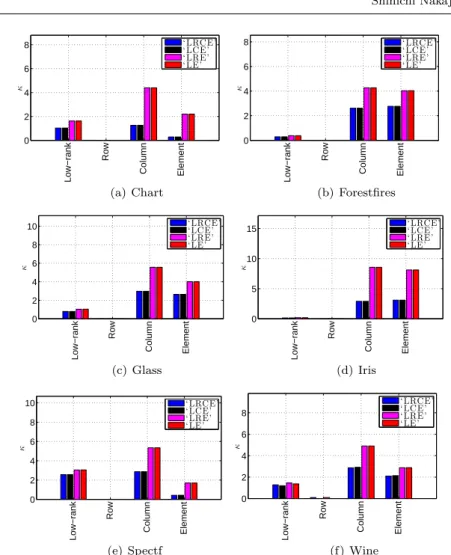
5 Experimental Results
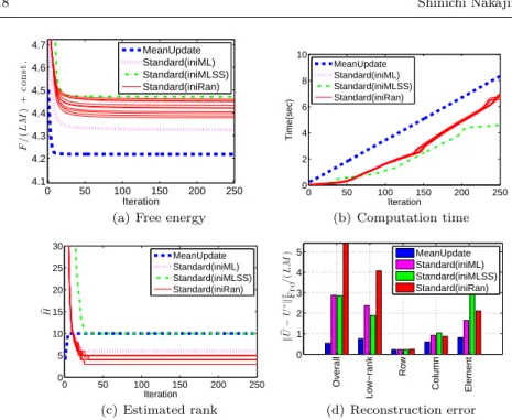
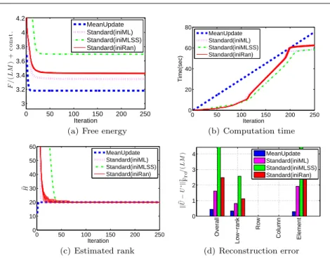
In this section, we first experimentally compare the performance of the MU algo- rithm and the standard VB iteration. Then, we test the model selection ability of SAMF, based on the free energy comparison. After that, we demonstrate the usefulness of the flexibility of SAMF on benchmark datasets and in a real-world application.
5.1 Mean Update vs. Standard VB
We compare the algorithms under the following model: V = ULRCE+E,