学術雑誌掲載論文等

A uthor(s )

Unami, K oichi; Mohawesh, Osama

C itation

S tochastic E nvironmental R esearch and R isk A ssessment

(2018)

Is s ue D ate

2018-03-05

UR L

http://hdl.handle.net/2433/229528

R ig ht

©

T he A uthor(s) 2018. T his article is distributed under the

terms of the C reative C ommons A ttribution 4.0 International

L icense (http://creativecommons.org/licenses/by/4.0/), which

permits unrestricted use, distribution, and reproduction in any

medium, provided you give appropriate credit to the original

author(s) and the source, provide a link to the C reative

C ommons license, and indicate if changes were made.

T ype

J ournal A rticle

ORIGINAL PAPER

A unique value function for an optimal control problem of irrigation

water intake from a reservoir harvesting flash floods

Koichi Unami1 • Osama Mohawesh2

ÓThe Author(s) 2018. This article is an open access publication

Abstract

Operation of reservoirs is a fundamental issue in water resource management. We herein investigate well-posedness of an optimal control problem for irrigation water intake from a reservoir in an irrigation scheme, the water dynamics of which is modeled with stochastic differential equations. A prototype irrigation scheme is being developed in an arid region to harvest flash floods as a source of water. The Hamilton–Jacobi–Bellman (HJB) equation governing the value function is analyzed in the framework of viscosity solutions. The uniqueness of the value function, which is a viscosity solution to the HJB equation, is demonstrated with a mathematical proof of a comparison theorem. It is also shown that there exists such a viscosity solution. Then, an approximate value function is obtained as a numerical solution to the HJB equation. The optimal control strategy derived from the approximate value function is summarized in terms of rule curves to be presented to the operator of the irrigation scheme.

Keywords Optimal control problemValue functionHamilton–Jacobi–Bellman equationViscosity solution Irrigation schemeReservoir operation

1 Introduction

A stock-and-flow structure is a key concept in economics as well as in water resource management. Stocks of water in reservoirs, such as dams, aquifers, lakes, ponds, and tanks, regulate flows of water, which are intrinsically uneven and uncertain (Borgomeo et al.2014; Zhang and Babovic 2011). Stochastic processes and control theories have been applied to water resource management problems in both the design and operation stages (Leroux and Martin

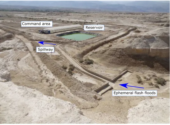
2016; Cui and Schreider2009; Zhao et al.2014; Pelak and Porporato2016; Basinger et al.2010). An extreme case is being studied in a harsh environment, where a small reservoir is constructed to collect ephemeral water flows from flash floods in order to fully irrigate perennial plants, as shown in Fig.1 (Unami et al. 2015). The structure

harvesting flash floods consists of a gutter cutting across a 16 m wide valley bottom and a conveyance channel of 60 m long to guide the water to the reservoir. The con-veyance channel is equipped with a spillway to release excess backwater from the reservoir. Operation of the reservoir involves an optimal control problem considering the inherently stochastic occurrence of flash floods, while the operator can make decisions on the intake flow rate from the reservoir for irrigation. The entire irrigation scheme, which consists of a reservoir with flash flood harvesting facilities and a command area of plant cultiva-tion, is so small that the decision maker has perfect information. The water dynamics in the irrigation scheme is modeled as a set of stochastic differential equations (SDEs) representing the water balance in the reservoir as well as the uncertain occurrence and intensity of flash floods and droughts. The performance index to be minimized is the expected deficiency of water in the future. In the present paper, we attempt to establish well-posed-ness for such an optimal control problem with mathemat-ical rigor, which is lacking in earlier practmathemat-ical papers on relevant topics (Unami et al. 2013, 2015; Sharifi et al.

2016).

& _{Koichi Unami}

[email protected]

1 _{Graduate School of Agriculture, Kyoto University,}

Kyoto 606-8502, Japan

2

Faculty of Agriculture, Mutah University, Karak 61710, Jordan

In the context of dynamics programming, the Hamilton– Jacobi–Bellman (HJB) equation governs the value function from which an optimal control strategy is derived for a time-continuous problem. The versatility of the HJB equation is evident as its industrial applications are so vast, covering the fields of population dynamics (Guo and Sun

2005), financial engineering (Junca 2012; Leach et al.

2007; Bo et al. 2013), aircraft flight mechanics (Almgren and Tourin2015), climate risk assessment (Chaumont et al.

2006), and energy systems (Sieniutycz2009,2012,2015). The notion of viscosity solutions is a powerful vehicle for approaching the HJB equation, which is nonlinear and degenerate in most cases, and comparison theorems are fundamental in discussing uniqueness and stability of solutions (Fleming and Soner 2006; Kawohl and Kutev

2007; Ishii1987; Ishii and Lions1990; Crandall and Lions

1983). Peron’s method is a standard means of constructing viscosity solutions (Crandall et al. 1992). However, the HJB equation derived from the optimal control problem considered herein encounters some difficulties. The com-parison theorems known thus far are not applicable because of irregular conditions imposed when the reservoir is empty or full. Therefore, special auxiliary functions are sought to establish a comparison theorem, which guaran-tees the uniqueness of a continuous viscosity solution to the HJB equation with a relaxed Hamiltonian. Another theo-rem is also proven to show the existence of the viscosity solution as well as to justify a numerical approach,

embedding a space of weak solutions into the space of viscosity solutions, in a manner analogous to a previous study dealing with one-dimensional stationary Hamilton– Jacobi equations of first order (Guermond and Popov

2008).

An approximate value function obtained as a numerical solution to the HJB equation yields the optimal control strategy in the real world. Concurrent use of the finite difference and finite element methods is a promising dis-cretization technique for nonlinear and degenerate partial differential operators. The optimal control strategy is the maximizer of a characteristic function depending on the value function. Assuming that the control strategy derived from the approximate value function is optimal, it is summarized in terms of rule curves for reservoir operation (Senga1991; Khan et al. 2012; Moghaddasi et al. 2013), and a simplified chart is presented to the operator for actual implementation. This is an innovative demonstration test in the prototype irrigation scheme based on a rigorous mathematical foundation.

As usual, the notationsC,C1,C2, andC1 shall be used for the sets of continuous and continuously differentiable functions.

2 Formulation of the optimal control

problem

A stochastic model is developed for water dynamics in the irrigation scheme. Then, an optimal control problem is formulated with a performance index to be minimized, in order to deduce the optimal control strategy for irrigation water intake from the reservoir harvesting flash floods.

2.1 Stochastic model for water dynamics

The dynamics of the storage volumeXt of the reservoir at

timet is governed by the water balance equation

dXt¼ðQin Qout uÞdt ð1Þ

whereQin is the inflow rate of the harvested flash flood,

which is equal to the runoff discharge of the flash flood after subtracting the rate of overflow from the spillway, Qoutis the outflow rate due to evaporation and seepage, and

uis the intake flow rate as a control variable constrained in a setUof admissible controls. A virtual variableYtreferred

to as the water flow index is considered to model the dynamics ofQin andQout. The one-dimensional Langevin

equation is assumed to governYt as

dYt¼ rYtdtþ

ffiffiffiffiffiffi

2D p

dBt ð2Þ

whereris a reversion coefficient,D is a diffusion coeffi-cient, andBt is the standard Brownian motion (Øksendal

2007). The advantages of using this virtual model (2) are capability in comprehensively representing the stochastic flow rate dynamics of flash floods as well as the occurrence of dry spells. A non-decreasing functionQinðyÞis assumed

to define the relationship betweenYtandQin, whileXtand

Yt determine Qout with another function Qoutðx;yÞ. The

storage volume Xt of the reservoir is assumed to almost

surely not exceed its capacity V, because of the well-functioning spillway. It is also trivial that Xt cannot

decrease when it is equal to 0. Consequently, the domain of Xtis restricted to the closed interval 0½ ;VŠ, as is common in

most reservoir operation problems. Consequently, (1) is rewritten as

dXt¼a Xð t;Yt;uÞdt ð3Þ

with

a x_ð ;y;u_{Þ ¼}

0_^ðQinð Þy Qoutðx;yÞ uÞ ifx¼V

Qinð Þy Qoutðx;yÞ u if 0\x\V

0_{_}ðQinð Þy Qoutðx;yÞ uÞ ifx¼0

8

<

:

ð4Þ

where^and_represent the minimum and the maximum, respectively. A target flow rateQtrgof irrigation water as a

function of the timet is set within the maximum capacity

of the intake facility, e.g., a pump. Depending on the fea-sibility of intake from the reservoir, the admissible setUis prescribed as

U_¼ 0;Qtrg

ifXt[0 orQ_trgQ_in Q_out

0

f g ifXt¼0 andQtrg[Q_in Q_out

: ð5_Þ

2.2 Performance index and HJB equation

The current timesis assumed to be in an irrigation period 0;T

½ Þ (T\1). The performance index Juðs;x;yÞ at time

t_¼s with storage volume Xs¼x and water flow index

Ys¼yis defined as

Ju_ðs;x;y_{Þ ¼}Es;x;y

Z T

s

f tð;u tð;Xt;YtÞ;YtÞdtþV XT

ð6_Þ

where Es;x;y _{represents the expectation with respect to the}

probability law of the stochastic processes starting at point s;x;y

ð Þ, and f is a bounded non-negative penalty function evaluating the departure of the actual intake flow rate u from the target Qtrg. The value XT at the end of the

irri-gation period is the bequest to be maximized. The choice of u is optimized to attain the infimum of Ju_ðs;x;y_Þ. It is assumed thatuis a Markov control, the choice of which at timetdepends only on the current values ofXtandYt. The

infimum U¼U_ðs;x;y_Þ of Ju_ðs;x;y_Þ exists because f0 and 0V XTV, and is referred to as the value

func-tion. The controluattaining_Uis referred to as the optimal control. Therefore,

U_ðs;x;y_{Þ ¼}Ju_ðs;x;y_Þ

¼Es;x;y

Z T

s

f tð;uðt;Xt;YtÞ;YÞdtþV XT

:

ð7_Þ

As mentioned in Chapters IV and V of Fleming and Soner (2006) including the verification theorem, the HJB equation

o_U

o_s þa x;y;u

ð Þo_oU

x ry

o_U

o_yþD

o2_U

o_y2 þf sð ;u;yÞ

¼inf

u2U

o_U

os þa xð ;y;uÞ

o_U

ox ry

o_U

oyþD

o2_U

oy2 þf sð ;u;yÞ

¼0

ð8_Þ

governs the value function_Uand the optimal controlufor s;x;y

ð Þ in the set G_¼½0;T_{Þ ð}0;V_Þ R, with the ter-minal condition

UðT;x;y_{Þ ¼}V x: ð9_Þ

functionUshould be understood as a viscosity solution to the HJB Eq. (8), which is degenerating. The optimal con-trolu at any point inGis obtained as

u_¼arg max

u2U

wðu_{Þ ð}10_Þ

wherewis the characteristic function defined by

w_ðu_{Þ ¼}w_ðu;t;x;y;UÞ ¼uoU

ox fðt;u;yÞ: ð11Þ

Then, the HJB equation (8) is rewritten as

o_U

os þDQ

o_U

ox ry

o_U

oyþD

o2_U

oy2 wðu

_{Þ ¼0 ð12Þ}

where

DQ_¼

u_^ðQin QoutÞ ifx¼V

Qin Qout

ð Þ if 0\x\V

u_{_}ðQin QoutÞ ifx¼0

8

<

:

: ð13Þ

A penalty function is chosen as

f_ðt;u;y_{Þ ¼} cðyÞ ifu6¼QtrgðtÞ 0 ifu_¼QtrgðtÞ

ð14Þ

where c is a positive bounded weight depending on the water flow indexy, which is assumed here to be

c_¼ Qtrg

1_þexp_ðy K_Þ ð15Þ

whereK is a model parameter, which will be determined from physical data observed in the real world (Sect.5). For a feasible operational flow rateQpof the intake facility, the

irrigation period 0_½ ;T_Þis divided intoN_þ1 non-irrigation hours I2i¼½t2i;t2i_þ1Þ and N irrigating hours

I2iþ1 ¼½t2iþ1;t2iþ2Þ, where Qtrg¼0 and Qtrg¼Qp,

respectively, so that 0_½ ;T_{Þ ¼}½t0;t2Nþ1Þ ¼ [ 2N

k¼0Ik. This

par-tition of the entire irrigation period into a sequence of time intervals reduces the original problem into a sequence of the HJB equations with Hamiltonians independent of time. Under the above-mentioned conditions, it is easy to verify the boundedness of_U:

Remark 1 For anys_2½0;T_Þ, 0U_ðT s_Þmax Qp

þV: ð16_Þ

WhenQtrg¼Qp, (10) and (11) are reduced to

u_¼

0 if Qp

o_U

o_x\ c

8u₂U ifQp

o_U

ox¼ c

Qp ifQp

o_U

o_x [ c

8

> > > > > <

> > > > > :

ð17Þ

and

w¼Qp

o_U

ox_ c: ð18Þ

Otherwise, these two equations are reduced to

u_¼0 _ð19_Þ

and

w¼ c: ð20Þ

The optimal control u may not be unique, as in (17). However, eliminating u reduces the HJB Eq. (12) with (18) and (20) to obtain

o_U

os þð0^ðQin QoutÞÞ

o_U

ox ry

o_U

oyþD

o2_U

oy2 þc¼0 if Qp

o_U

ox c

o_U

o_s þ 0^ Qin Qout Qp

oU

o_x ry

o_U

o_yþD

o2_U

o_y2 ¼0 if Qp

o_U

o_x c

8

> > <

> > :

if x_¼V; ð21_Þ

o_U

os þðQin QoutÞ

o_U

ox ry

o_U

oyþD

o2_U

oy2 þc¼0 if Qp

o_U

ox c

o_U

o_s þ Qin Qout Qp

oU

o_x ry

o_U

o_yþD

o2_U

o_y2 ¼0 if Qp

o_U

o_x c

8

> > <

> > :

if 0\x\V; ð22Þ

and

o_U

os þð0_ðQin QoutÞÞ

o_U

ox ry

o_U

oyþD

o2_U

oy2 þc¼0 if Qp

o_U

ox c

o_U

os þ 0_ Qin Qout Qp

oU

ox ry

o_U

oyþD

o2_U

oy2 ¼0 if Qp

o_U

ox c

8

> > <

> > :

3 Uniqueness of viscosity solution

to the HJB equation

For each non-negative integerk2N, the temporal vari-able is inverted as

s¼tkþ1 s2ð0;tkþ1 tkŠ; ð24Þ

and the value function_U¼Uðs;x;y_Þis defined on the set Gk¼ð0;tk_þ1 tkŠ ½0;VŠ R. Then, the HJB

equa-tions (21), (22), and (23) is further rewritten as

o_U

o_sþHðs;x;U;rU;r rUÞ ¼0 ð25Þ

wherex_¼ x y

, andH is the Hamiltonian defined as

H_ðs;x;w;p;M_{Þ ¼}H_ðs;x;p;M_Þ

¼_H^_{ðs;x;y;pxÞ þrypy Dl}

yy ð26Þ

with

^

Hðs;x;y;pxÞ ¼

a_ðx;y;0_Þpx c if Qppxþc0

a x;y;Qp

px if Qppxþc0

ð27Þ

and

a_ðx;y;Q_{Þ ¼}

0^ðQinð Þy Qoutðx;yÞ QÞ if x¼V

Qinð Þy Qoutðx;yÞ Q if 0\x\V

0_{_}ðQinð Þy Qoutðx;yÞ QÞ if x¼0

8

<

:

ð28_Þ

where p_¼ px py

and M_¼ lxx lxy lyx lyy

. However, the

discontinuity appearing in (28) when x_¼0 and x_¼V hinders the comparison theorem, which holds if the func-tiona_ðx;y;Q_Þis relaxed as

agðx;y;QÞ

¼

V x

g aðV g;y;QÞ þ 1 V x

g

aðV;y;QÞ ifxV g

aðx;y;QÞ ifx¼g\x\V g

1 x

g

a_ð0;y;Q_{Þ þ}x

ga g;ð y;QÞ ifxg

8 > > > > > < > > > > > :

ð29_Þ whereg is a small positive relaxation parameter, so that agðx;y;QÞ uniformly approaches aðx;y;QÞ as g!0.

Henceforth, thisagðx;y;QÞwill be used in (27) instead of

a_ðx;y;Q_Þ. The definitions of a x_ð ;y;u_Þ and DQ will be accordingly revised asagðx;y;uÞandDQg in (4) and (13),

respectively. The assertion of Remark 1 is still valid for the relaxed case.

Remark 2 H^ðs;x;y;pxÞwith the relaxed (29) is Lipschitz

continuous in eachIkwith respect tos,x, andy.

Now, we move on to viscosity solution to the relaxed HJB equation. A real-valued functionUdefined on a setE is called upper semi-continuous, if for any_ðs;x_{Þ 2}ER3

and anye[0 there existsdsuch thatUðs0;x0Þ\Uðs;xÞ þ

e for all _ðs0_;x0_{Þ 2B}

dðs;xÞ \E, where Bdðs;xÞ represents

the d-neighborhood of_ðs;x_Þ. Similarly, it is called lower semi-continuous in the case where the inequality is replaced by U_ðs0_;x0_Þ[Uðs;xÞ e. Let USC Eð Þ and

LSC E_{ð Þ} denote the sets of all upper and lower semi-con-tinuous functions defined onE, respectively. The upper and lower semi-continuous envelopes UU and UL of a real-valued function_UonGkare defined as

UU_ðs;x_{Þ ¼} lim sup

s0;x0

ð Þ!ðs;xÞU

s0;x0

ð Þ ð30_Þ

and

UL_ðs;x_{Þ ¼} lim inf

s0;x0

ð Þ!ðs;xÞU s 0_;x0

ð Þ; ð31Þ

respectively. Note thatUL

2USCð ÞGk andUL2LSCð ÞGk .

ForUU

2USCð ÞGk , being a viscosity sub-solution to (25)

implies that

ow

o_sþHðs;x;w;rw;r rwÞ 0 atðs;^x^Þ 2Gk ð32Þ

for any test functionw₂C2ð ÞGk , such that

w_UU inGk; w¼UU atðs;^x^Þ: ð33Þ

For_UL

2LSCð ÞGk , being a viscosity super-solution to (25)

implies that

o_w

o_sþHðs;x;w;rw;r rwÞ 0 atðs;^x^Þ 2Gk ð34Þ

for any test functionw₂C2 _G

k

ð Þ, such that

wUL _inG

k; w¼UL atðs;^ x^Þ: ð35Þ

If _UU _{is a viscosity sub-solution and}

UL is a viscosity super-solution, then Uis called a viscosity solution.

We firstly discuss the continuity of viscosity solutions, which are value functions of the optimal control problem, ats_¼0.

Theorem 1 Suppose that Uv is a bounded viscosity

solution to(25)with(29)and that_UU_vð0;x_{Þ ¼U}L_vð0;x_Þfor x_2½0;V_Š R. If Uvð0;xÞ ¼UUvð0;xÞ ¼U

L

vð0;xÞ as a

function ofx is continuous in_½0;V_Š R, then lim

s0;x0

ð Þ!ð0;xÞUv s 0_;x0

ð Þ Uvð0;xÞ

j j ¼0: ð36_Þ

Proof _{For s}0₂½_0;tkþ1 tkŠ andx02½0;VŠ R, it holds

Uvðs0;x0Þ Etkþ1 s

0_;x0 Z tkþ1

tkþ1 s0

f t;u;Y_t0dt_þUvð0;X0ð0;uÞÞ

ð37_Þ

with

X0_ðs;u_{Þ ¼} X 0

tkþ1 s

Y_t0

kþ1 s

¼x0_þ

Z tkþ1 s

tkþ1 s0

agðXt;Yt;uÞ

rYt

dt

þ

Z tkþ1 s

tkþ1 s0

0

ffiffiffiffiffiffi

2D p

dBt ð38Þ

for any admissibleu, becauseUvis a value function of the

optimal control problem. For any e[0, there exists an

admissibleu~such that

Uvðs0;x0Þ

þe[Etkþ1 s0;x0

Z tkþ1

tkþ1 s0

f t;u~;Y_t0dt_þUvð0;X0ð0;u~ÞÞ

:

ð39_Þ

With the chosen penalty function (14), the first part of the expectation in the right hand side of (39) is evaluated as

Etkþ1 s0;x0

Z tkþ1

tkþ1 s0

f t;u~;Y_t0dt

Qtrgs0; ð40Þ

and then subtractingUvð0;xÞfrom the inequalities (37) and

(39) leads to

Uvðs0;x0Þ Uvð0;xÞ

j j Etkþ1 s0;x0

Z tkþ1

tkþ1 s0

f t;u~;Y_t0dt

þUvð0;X0ð0;u~ÞÞ Uvð0;xÞ

Qtrgs0þ Etkþ1 s

0_;x0

Uvð0;X0ð0;u~ÞÞ Uvð0;xÞ

½ Š

Qtrgs0þEtkþ1 s

0;x0

Uvð0;X0ð0;u~ÞÞ Uvð0;xÞ

j j

½ Š

ð41_Þ

for anyx_2½0;V_Š R. By the definition (38)

lim

s0;x0

ð Þ!ð0;xÞUv 0;X 0_ð0;u~Þ

ð Þ Uvð0;xÞ

j j ¼0 ð42Þ

and therefore (36) holds. h

The following comparison theorem coupled with The-orem 1 proves the uniqueness of viscosity solutions of (25) with (29).

Theorem 2 Suppose that U12USCð ÞGk is a bounded

viscosity sub-solution to (25) with (29) and that _U22

LSCð ÞGk is a bounded viscosity super-solution to(25)with

(29). Then,

sup

s;x

ð Þ2Gk

U1ðs;xÞ U2ðs;xÞ

ð Þ ¼ sup

n2½0;VŠR

U1ð0;nÞ U2ð0;nÞ

ð Þ:

ð43_Þ

Proof _{We opt for proof by contradiction in two stages.}

Firstly, an auxiliary function_Wis defined as Wðs;x;r;nÞ ¼U1ðs;xÞ U2ðr;nÞ

1 2djs rj

2 1

2ekx nk

2

u r_{ð Þ ð}44_Þ

wheren_¼ n

f

, andu s_{ð Þ 2}C1ð½0;tkþ1 tkŠÞis a

func-tion satisfyingu s_{ð Þ} 0 andu s_{ð Þ ¼}0 ifs_¼0. Two points

s;x

ð Þand r; nof_{Gk are assumed to maximizeWas}

W s;x;r; n

¼ sup

s;x

ð Þ;ðr;nÞ2_GkW s;

x;r;n

ð Þ: ð45_Þ

Then, the inequality

U1ðs;xÞ U2 r; n

1 2djs rj

2 1

2e x n

2

¼W s;x;r; n

þu_{ð Þ}r W r; n; r; n

¼U1 r; n U2 r; n

ð46Þ

leads to evaluations

s r

j j ffiffiffiffiffiffiffiffiK1d

p

andx n

ffiffiffiffiffiffiffi

K1e

p

ð47_Þ

whereK1 is a non-negative constant given by

K1¼4 max

s;x

ð Þ2_GkðjU1ðs;xÞj;jU2ðs;xÞjÞ

\þ 1: ð48Þ

Assume that s[0 and r[0. We set a smooth function

v_ðs;x_Þas

v_ðs;x_{Þ ¼} 1 2djs rj

2

þ1 2e x

n

2

ð49_Þ

which turns out to be a test function for a viscosity sub-solution because

U1ðs;xÞ vðs;xÞ ¼W s;x;r; nþU2 r; nþuð Þr

ð50_Þ

and therefore

s;x

ð Þ 2arg max

s;x

ð Þ2Gk

U1ðs;xÞ vðs;xÞ

f g: ð51_Þ

ov

o_sþHðs;x;rv;r rvÞ ¼

1 dðs rÞ þH s;x;1

e x n ;1 eI

¼1_dðs r_Þ

þ_H^ _s;x;1 e x

n

þry 1 e y

f

_D

e 0 at_ðs;x_Þ:

ð52_Þ

An eligible functionu sð Þis chosen here as

u s_{ð Þ ¼}1 2bs

2

þ2D_e s _ð53_Þ

withb[0, to set another smooth functionv^ðs;xÞas

^

vðr;nÞ ¼ ₂1 djs rj

2

þ₂1

ekx nk

2

þu r_{ð Þ}

ð54_Þ

which turns out to be a test function for a viscosity super-solution because

U2ðr;nÞ v^ðr;nÞ ¼ Wðs;x;r;nÞ þU1ðs;xÞ ð55Þ

and therefore

r;n

2arg min

s;x

ð Þ2Gk

U2ðr;nÞ v^ðr;nÞ

f g: ð56_Þ

This implies that

ov^

o_rþHðr;n;rv^;r rv^Þ ¼ br

2D e þ

1 dðs rÞ þH r;n;1

eðx nÞ; 1 eI

¼ br 2D e þ

1 dðs rÞ þ_H^ _r;n;1

eðx nÞ

þrf 1 eðy fÞ

þD_e 0 at r; n

:

ð57_Þ

Comparing (52) and (57) yields

br_þ1 er y

f2

_H^ _{r; n;} 1 e x

n

^ H s;x;1

e x n

: ð58_Þ

The left-hand side of (58) remains positive for any positive b,d, ande, while its right-hand side approaches to zero as d;e! þ0 because H^ is continuous, to yield a contradic-tion. Therefore,s¼0 orr¼0 or both.

Now, we prove

sup

s;x

ð Þ2Gk

U1ðs;xÞ U2ðs;xÞ

ð Þ sup

n2½0;VŠR

U1ð0;nÞ U2ð0;nÞ

ð Þ:

ð59_Þ

Assume that (59) is not true. Then, there exists a point sM;xM

ð Þ 2Gksuch that

U1ðsM;xMÞ U2ðsM;xMÞ

¼ sup

s;x

ð Þ2Gk

U1ðs;xÞ U2ðs;xÞ

ð Þ

[ sup

n2½0;VŠR

U1ð0;nÞ U2ð0;nÞ

ð Þ;

ð60_Þ

while one of the inequalities

U1ðs;xÞ U2ðs;xÞ sup

x2½0;VŠR

U1ð0;xÞ U2ð0;xÞ

ð Þ ifs¼0

U1 r;n U2 r;n sup

n2½0;VŠR

U1ð0;nÞ U2ð0;nÞ

ð Þ ifr¼0

8 > <

> :

ð61_Þ

holds. By the evaluations (47), it is possible to chooseeand d such that js rj þx n

q for any q[0. Then,

considering the properties of upper and lower semi-con-tinuous functions,qis chosen so that

U2ðs; xÞ U2 r; n\e₀ if s¼0

U1ðs; xÞ U1 r; n\e₀ if r¼0

ð62_Þ

for anye0[0. Adding (62) to (61) results in

U1ðs;xÞ U2 r; n sup

n2½0;VŠR

U1ð0;nÞ U2ð0;nÞ

ð Þ þe0

ð63Þ

to obtain

W s;x;r; n

¼U1ðs;xÞ U2 r; n

1 2djs rj

2 1

2e x n 2

u_{ð Þ}r

sup

n2_½0;V_ŠR

U1ð0;nÞ U2ð0;nÞ

ð Þ

þe0

1 2djs rj

2 1

2e x n

2

uð Þr

\ sup

s;x

ð Þ2Gk

U1ðs;xÞ U2ðs;xÞ

ð Þ þe0:

ð64_Þ

On the other hand,

WðsM;xM;sM;xMÞ ¼U1ðsM;xMÞ U2ðsM;xMÞ u sð ÞM

¼ sup

s;x

ð Þ2Gk

U1ðs;xÞ U2ðs;xÞ

ð Þ u sð ÞM :

ð65_Þ

W s;x;r; n

\ sup

s;x

ð Þ2Gk

U1ðs;xÞ U2ðs;xÞ

ð Þ þe0

¼WðsM;xM;sM;xMÞ þu sð Þ þM e0: ð66Þ

Another choice ofu s_{ð Þ}as

u sð Þ ¼1 2bs

2 _ð67Þ

withb[0 is also eligible and leads to

W s;x;r; n

\Wðs_M;x_M;s_M;x_MÞ ð68Þ

as b;e0! þ0. However, (68) contradicts (45) and thus

(59) is true. Consequently, we reach to (43). h

Remark 3 _{If there is a viscosity solution to (25) with (29)}

satisfying a specified continuous initial condition in the sense of Theorem 1, then its uniqueness and continuity are direct consequences of Theorem 2.

4 Existence of viscosity solution to the HJB

equation

A weak solution to the HJB equation (25) with (29) from a specified initial condition is considered in order to show the existence of a viscosity solution as well as to provide a framework for approximate numerical solution.

Transformation of the independent variableytozwith z_¼tan 1 ffiffiffiffiffir

2D

p

y

makes the domain bounded. Indeed,Gk

is mapped to G_k¼ð0;tkþ1 tkŠ XxXz, where Xx¼

0;V

ð ÞandXz¼ð p=2;p=2Þ. LetXsdenote 0ð ;tk_þ1 tkÞ.

Then, the HJB equation (25) is formally transformed into

o_U

o_sþH^ s;x;

ffiffiffiffiffiffi

2D r

r

tanz;oU

ox

!

þrsinzcosz 1_þcos2zoU

o_z

r 2cos

4_zo 2

U

o_z2

¼0; ð69_Þ

but U at each s₂ð0;tkþ1 tkŠ shall be sought in the

function spaceH1

xz, which is completed with the norm

U k kH1

xz¼

Z

Xz

U k kH1_X

x

ð Þdzþ

Z

Xx

U k kH1_X

z

ð Þdx ð70Þ

where

U k kH1_X

ð Þ¼

ffiffiffiffiffiffiffiffiffiffiffiffiffiffiffiffiffiffiffiffiffiffiffiffiffiffiffiffiffiffiffiffiffiffiffiffiffiffiffiffiffiffi Z

X

U2þ o_oU 2! d* v u u

t ð71Þ

for _¼xorz, to satisfy the weak form

d ds Z Xx ^ wx Z Xz ^ wzUdzdx

¼ Z Xx ^ wx Z Xz

rw^zsin3zcoszþ

r 2cos

4_zow^z

oz

_o

U

oz

þw^zH^ s;x;

ffiffiffiffiffiffi

2D r

r

tanz;oU

ox

!!

dzdx

ð72_Þ

for any weights w^x2H1ð ÞXx and w^z2H1ð ÞXz , where

H1_{ð ÞX} is the Sobolev space equipped with the norm (71). For _¼sorxorz, it is known that there are embeddings H1ð Þ !X CBð ÞX and H1ð Þ !X C X, where CBð ÞX is the set of all bounded continuous functions on a domain X, and C X is the set of all bounded uniformly con-tinuous functions on a domain _X. Both of CBð ÞX and

C _X

are Banach spaces equipped with the uniform norm, and C X is a closed subspace of CBð ÞX (Adams and Fournier2003). LetCB Gk

denote the set of all bounded continuous functions on G_k, which is a Banach space equipped with the uniform norm k kU 1¼ sup

s;x;z

ð Þ2G

k

U j j.

Consider the function g of w^x, w^z, and UðjÞ with time incrementdsas

g w^x;w^z;U_ðjÞ¼

Z Xx ^ wx Z Xz ^

wzU_ðjÞdzdx

ds Z Xx ^ wx Z Xz

F w^z;U_ðjÞ

dzdx ð73Þ

where

Fðw^z;UÞ ¼ rw^zsin3zcoszþ

r 2cos

4_zow^z

oz

_o

U

oz

þw^zH^ s;x;

ffiffiffiffiffiffi

2D r

r

tanz;oU

ox

!

:

ð74Þ

For fixedw^zandU_ðjÞ,gis a continuous linear functional on H1ð Þ_Xx . For fixed w^x and UðjÞ, g is a continuous linear functional on H1ð ÞXz . Applying the Riesz representation

theorem (Adams and Fournier2003) twice, gis identified with another functionUðjþ1Þ2Hxz1. Starting from an initial

value _Uð0Þ, iterations UðjÞ

j¼1;2;3... with ds¼s=Ns and

Ns1 yield the Riemann sum

Z Xx ^ wx Z Xz ^

wzUðNsÞdzdx¼ Z Xx ^ wx Z Xz ^

wzUð0Þdzdx

s 1 Ns

X

Ns 1

l¼0

Z Xx ^ wx Z Xz

F w^z;U_ðl_Þ

dzdx:

ð75Þ

Z Xx ^ wx Z Xz ^

wzUdzdx¼

Z Xx ^ wx Z Xz ^

wzU_ð0Þdzdx

s Z Xx ^ wx Z Xz

Fðw^z;UÞdzdx ð76Þ

asNsapproaches þ1, which is consistent with (72).

Remark 4 _{There exists at least one solution Uw¼}

Uwðs;x;zÞto the initial value problem (72) with an initial

value_Uð0Þ2H1xz. Here,Uw2Hxz1 for anys2ð0;tk_þ1 tkŠ

andUw2CBð ÞXs for any ðx;zÞ 2XxXz, implying that

Uw2CB Gk

.

The following theorem asserts that the above-mentioned weak solution accords with the viscosity solution to (25).

Theorem 3 Suppose thatUv¼Uvðs;xÞ ¼Uvðs;x;yÞis a

bounded viscosity solution to(25)with(29)satisfying the initial condition _Uvð0;xÞ ¼Uvð0;x;yÞ ¼

Uð Þ0 x;tan 1 ffiffiffiffiffiffiffiffi2rDy

p

for any x_ð ;z_{Þ 2}XxXz and that

Uw¼Uwðs;x;zÞ is a weak solution to(72)with (29)

sat-isfying the same initial condition. Then,

Uvðs;x;yÞ ¼Uw s;x;tan 1

ffiffiffiffiffiffiffiffiffi r 2Dy r

ð77Þ

in Gk.

Proof _LetUU

v andU

L

v be the upper and lower

semi-con-tinuous envelopes ofUv, respectively. Namely,UUv andU L v

are the viscosity sub-solution and the viscosity super-so-lution, respectively. From Theorem 1,

UUvð0;xÞ ¼U L

vð0;xÞ ¼Uvð0;xÞ 2CBð½0;VŠ RÞ ð78Þ

whereCBð½0;VŠ RÞis the set of all bounded continuous

functions on _½0;V_{Š R}. There exists a sequence Uð Þn_ðs;x;zÞ

C1 G_k\C2ð ÞXz converging to Uw.

Namely, for anye[0, there exists a natural number N₁

such that

Uwðs;x;zÞ Uð Þnðs;x;zÞ

_H1

xz

\e ð79Þ

for any n[N₁ at all s2ð0;t_kþ1 t_kŠ. Because of the

embeddings H1ð Þ !Xx C Xx

and H1ð Þ !Xz CBð ÞXz ,

there exists another natural numberN2, such that

Uwðs;x;zÞ Uð Þnðs;x;zÞ

1\e ð80Þ

for any n[N₂ at all s2 0;t_k

þ1 tk

ð Š. Consequently, Uð Þn_ðs;x;zÞ

becomes a Cauchy sequence converging to a limit _Ucðs;x;zÞ in CB Gk

, and thus _Uwðs;x;zÞ ¼

Ucðs;x;zÞinGk. Furthermore, for anyd[0, there exists a

natural numberN3 such that

o_Uð Þn

o_s þH s;x;

ffiffiffiffiffiffi

2D r

r

tanz;Uð Þn_;rUð Þn_{;r rU}ð Þn

! \d

ð81_Þ

for anyn[N₃inG

k. For eachn, letd n

ð Þ

i (i¼1;2) be real

numbers such that

dð Þ₁n ¼inf d0d ffiffiffi

s

p

[UU v s;x;

ffiffiffiffiffiffi 2D r r tanz !

Uð Þn_ðs;x;zÞ ( )

ð82_Þ

and

dð Þ₂n _¼sup d0d ffiffiffi

s

p

\UL v s;x;

ffiffiffiffiffiffi 2D r r tanz !

Uð Þn_ðs;x;zÞ ( ) :

ð83_Þ

Then, test functionswð Þ_in are chosen as

wð Þ_in _¼wð Þ_in_ðs;x;y_Þ

¼Uð Þn s;x;tan 1

ffiffiffiffiffiffiffiffiffi r 2Dy r

þdð Þin

ffiffiffi

s p

ð84Þ

so that

wð Þ₁n UUv inGk; w n

ð Þ

1 ¼U

U

v atðs^1;x^1Þ ð85Þ

and

wð Þ₂n UL

v inGk; w

n

ð Þ

2 ¼U

L

v atð^s2;x^2Þ ð86Þ

for some ð^si;x^iÞ 2Gk. This implies that w n

ð Þ

i are indeed

eligible for test functions of viscosity sub-solutionUUv and

viscosity super-solution_UL

v, resulting in

o_wð Þn

1

o_s þH s^1;x^1;w

n

ð Þ

1 ;rw

n

ð Þ

1 ;r rw

n

ð Þ

1

¼oU ðn_Þ

os þH s^1;x^1;U

ðnÞ_;rUðnÞ_{;r rU}ðnÞ

þd n ð Þ 1 ffiffiffi s

p 0 _ð87_Þ

and

owð Þ₂n

o_s þH s^2;x^2;w

n

ð Þ

2 ;rw

n

ð Þ

2 ;r rw

n

ð Þ

2

¼oU ðnÞ

o_s þH s^2;x^2;U

ðnÞ_;rUðnÞ_{;r rU}ðnÞ

þd n ð Þ 2 ffiffiffi s

p 0 _ð88_Þ

at respectiveðs^i;x^iÞ. In order to satisfy (87) and (88),d n

ð Þ

i

UUvðs;x;yÞ ¼U L

vðs;x;yÞ ¼Uc s;x;tan 1

ffiffiffiffiffiffi

r 2D

r

y

ð89_Þ inGk, and thus (77). h

5 Application with numerical demonstration

A prototype irrigation scheme including a reservoir for harvesting flash floods is being developed at the Agricul-tural Research Station of Mutah University, located in the Lisan Peninsula of the Dead Sea near the town of Ghor al Mazrah in Jordan. The model parameters are determined from the physical dimensions of the structures as well as from hydro-meteorological observation conducted from September 27th, 2014 through September 22nd, 2016. Indeed, the reservoir consists of two sections: a 300 m3 section enclosed in a greenhouse, and a 700 m3section, the surface of which is exposed to open air. Once a flash flood is harvested in the open section, the water is immediately transferred to the closed section if there is room. Therefore, the sections are regarded collectively as a single reservoir ofV = 1000 m3withQoutðx;yÞvarying in the x-direction.

The irrigation period 0_½ ;T_Þis set as 5.25609105min of a

non-leap year from May 1st through April 30th. No flash flood is expected during the months from May through October. The period from 08:00 a.m. through 08:12 a.m. is prescribed as the irrigation hours for every day throughout the irrigation period. Without loss of generality, the dif-fusion coefficient D is assumed to be unity. In the two consecutive winter rainy seasons of 2014–2015 and 2015– 2016 included in the observation period, there were 16 events of flash floods (10 events in 2014–2015 season and 6 events in 2015–2016 season), out of which 8 events (3 events in 2014–2015 season and 5 events in 2015–2016 season) yielded substantial harvesting. The model param-eter K represents the supremum of y, where there is no

inflow of flash flood to the reservoir, and its value is esti-mated to be 2.4165. The most likely value of the reversion coefficient in terms of the compatible transition probability density function is 0.0011421 per minute. The functions Qinð Þy and Qoutðx;yÞ are determined as shown in Fig.2.

The blue line in the figure indicatesQin in the unit of m3/

min during the wet months from November through April, identified from statistical analysis of the observed data as

Qinð Þ ¼y

60:000 if 58:181\y

18:305 logy 14:3833 if 3:7700\y58:181

27:641y 94:299 if 3:6000\y3:7700

3:6107ðy KÞ2:1767 ifK\y3:6000

0:0000 ifyK

8

> > > > <

> > > > :

;

ð90_Þ whileQin0 during the dry months from May to October.

Seepage is negligible because of plastic sheets covering the bottom of the reservoir, and the closed section is free from evaporation. Evaporation from the water surface of the open section is estimated at 10=_ð1_þexp_ðy K_ÞÞmm/day., which is multiplied by the water surface area depending on x to yield Qoutðx;yÞ. Note that there is no significant

dif-ference in observed evaporation between the wet and dry months.

To approximately solve the HJB equation (72) with (29) from a specified initial condition and then to derive the optimal control strategy, a computational procedure is developed as follows. Thez-domain_Xz is divided into nz

sub-domains of equal lengthDz_¼p=nz. Thex-domainXx

is also divided into nx sub-domains of equal length

Dx_¼V=nx, and the unknownUis attributed to each node

x_¼iDx;z_¼kDz

f g as Ui;k. For discretization in the

z-di-rection, the finite element scheme developed by Unami et al. (2015) is applied to the weak form (72). For dis-cretization in the x-direction, the first-order upwind finite difference scheme is used. The mesh size_Dxis regarded as the relaxation parameter g. Then, the system of ordinary differential equations resulting from those discretization

Outflow discharge (m /day) Inflow dischar

g

e (m /min)

3 ₃

10

8

6

4

2

0

60

48

36

24

12

0

x x x x x

250 100 75 50 25 0 25 50 75 100 250

∞ ∞

− − − − − − K

y Q

Q_{out in}

: = : = : = : = : =1000 m

800 m 600 m 400 m 0-300 m

3 3 3 3

3

schemes is numerically solved in thes-direction using the Runge–Kutta method with a constant time step Ds to update the value of eachUi;k. The optimal control strategy

u is derived from the computedUi;k, according to (10). A

computational run with nx¼100, nx¼120, and Ds¼

1=60 minutes was completed within nine days and four hours using the supercomputer system of the Academic Center for Computing and Media Studies, Kyoto Univer-sity. Distribution of computed optimal control u is delin-eated in Figs.3, 4,5, 6 and 7 for the irrigation hours of

Day 0

8:11

8:10 8:09

8:08 8:07

8:06 8:05

8:04

8:03

8:02 8:01

8:00 8:00 8:00 8:00 8:00 8:00 8:00 8:00 8:00 8:00 8:00 8:00 8:00 8:00 8:00 8:00 8:00 8:00 8:00 8:00 8:00 8:00 8:00 8:00 8:00 8:00 8:00 8:00 8:00 8:00 8:00 8:00 8:00 8:00 8:00 8:00 8:00

−∞ −250 −100 75− −50 −25 0 25 50 75 100 250 ∞

1000

800

600

400

200

K

x

y

Q

= =

0

(m )

u

u

p Fig. 3 Distribution of computed

optimal controluduring irrigation hours on May 1st (Day 0)

Day 91

8:11

8:10 8:09

8:08 8:07

8:06 8:05

8:04

8:03

8:02 8:01

8:00

−∞ −250 −100 75− −50 −25 0 25 50 75 100 250 ∞

1000

800

600

400

200

K

x

y

Q

= =

0

(m )

u

u

p Fig. 4 Distribution of computed

optimal controluduring irrigation hours on July 31st (Day 91)

Day 182

8:11

8:10 8:09

8:08 8:07

8:06 8:05

8:04

8:03

8:02 8:01

8:00

−∞ −250 −100 75− −50 −25 0 25 50 75 100 250 ∞

1000

800

600

400

200

K

x

y

Q

= =

0

(m )

u

u

p Fig. 5 Distribution of computed

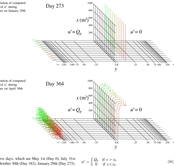
representative days, which are May 1st (Day 0), July 31st (Day 91), October 30th (Day 182), January 29th (Day 273), and April 30th (Day 364). The boundary between two adjacent cells ofu_¼0 andu _¼Qpin thex-ydomain for

eachs₂½0;t2iþ2 t2iþ1Þis marked as a segment in a

dif-ferent color at each time stage of 1-min intervals. If there is a surface ofxh such that

u_¼ Qp if x[xh 0 if x\x_h

ð91Þ

in thes–ydomain, the surface is referred to as a rule curve. Possibly due to the coarse discretization, oscillations in the delineated segments appear slightly in Figs. 3,4,5 and6

and more visibly neary_{¼ 1} in Fig.7. However, prac-tically significant rule curves can be extracted. The rule

Day 273

8:11

8:10 8:09

8:08 8:07

8:06 8:05

8:04

8:03

8:02 8:01

8:00

−∞ −250 −100 75− −50 −25 0 25 50 75 100 250 ∞

1000

800

600

400

200

K

x

y

Q

= =

0

(m )

u

u

p Fig. 6 Distribution of computed

optimal controluduring irrigation hours on January 29th (Day 273)

Day 364

8:11

8:10 8:09

8:08 8:07

8:06 8:05

8:04

8:03

8:02 8:01

8:00

−∞ −250 −100 75− −50 −25 0 25 50 75 100 250 ∞

1000

800

600

400

200

K

x

y

Q

= =

0

(m )

u

u

p Fig. 7 Distribution of computed

optimal controluduring irrigation hours on April 30th (Day 364)

MAY JUN JUL AUG SEP OCT NOV DEC JAN FEB MAR APR

Open part

Closed part

:Dry :Normal :Wet

curves are mostly monotonically increasing with respect to y, and, throughout the irrigation period, water should not be withdrawn from the reservoir under sufficiently wet con-ditions. The restriction on intake is strictest on Day 0 and is then relaxed as time evolves. Rule curves vanish after Day 182 under dry conditions.

The chart for the rule curves actually presented to the operator, which includes only three cases of water flow index y_¼ 3:2935_¼ 1:3629K_¼pffiffiffiffiffiffiffiffiffiffiffi2D=rtan_ðp=40_Þ andy_¼0, is shown in Fig.8. The operator has also been told that irrigation should not be performed during flash floods. On the other hand, the rule curve fory_¼ 3:2935 should be applied under much drier conditions.

6 Conclusions

A prototype irrigation scheme with a reservoir for har-vesting flash floods motivated the mathematical analysis of the present paper. A water dynamics model was con-structed based on practically acceptable assumptions, and the model parameters were determined from the observed data.

The optimal control problem formulated for the model was shown to have a unique value function, which solves the HJB equation in the viscosity sense. In other words, it was successfully demonstrated that the optimal control problem was well-posed. Skillful use of the properties of viscosity sub-solutions and viscosity super-solutions, as well as the choices of auxiliary functions, played key roles in the proofs of the non-trivial theorems. The innovative construction method for the weak solution rationalized the numerical approximation of the value function. The com-parison theorem, Theorem 2, is independent of Theorem 1 and is applicable to discontinuous viscosity solutions in general.

The rule curves for operation of the reservoir were numerically derived, suggesting that the optimal control is also unique. This is another remarkable outcome of the present study, because optimal control in a deterministic reservoir operation problem may be not unique, but may be arbitrary. Field verification of the optimal control strategy is being initiated in the real world, cultivating a perennial plant speciesPhoenix dactyliferain the irrigated command area.

Acknowledgements The authors are grateful to Prof. Hisashi Oka-moto at Gakushuin University for his valuable comments and sug-gestions. The present research was funded by Grants-in-Aid for Scientific Research Nos. 26257415 and 16KT0018 from the Japan Society for the Promotion of Science (JSPS).

Open Access This article is distributed under the terms of the Creative Commons Attribution 4.0 International License (http://

creativecommons.org/licenses/by/4.0/), which permits unrestricted use, distribution, and reproduction in any medium, provided you give appropriate credit to the original author(s) and the source, provide a link to the Creative Commons license, and indicate if changes were made.

References

Adams RA, Fournier JJF (2003) Sobolev spaces. Elsevier Science, Oxford

Almgren R, Tourin A (2015) Optimal soaring via Hamilton–Jacobi– Bellman equations. Optim Control Appl Methods 36:475–495 Basinger M, Montalto F, Lall U (2010) A rainwater harvesting system

reliability model based on nonparametric stochastic rainfall generator. J Hydrol 392:105–118

Bo L, Wang Y, Yang X (2013) Stochastic portfolio optimization with default risk. J Math Anal Appl 397:467–480

Borgomeo E, Hall JW, Fung F, Watts G, Colquhoun K, Lambert C (2014) Risk-based water resources planning: incorporating probabilistic nonstationary climate uncertainties. Water Resour Res 50(8):6850–6873

Chaumont S, Imkeller P, Mu¨ller M (2006) Equilibrium trading of climate and weather risk and numerical simulation in a Markovian framework. Stoch Environ Res Risk Assess 20(3):184–205

Crandall MG, Lions PL (1983) Viscosity solutions of Hamilton– Jacobi equations. Trans Am Math Soc 277(1):1–42

Crandall MG, Ishii H, Lions PL (1992) User’s guide to viscosity solutions of second order partial differential equations. Bull Am Math Soc 27(1):1–67

Cui J, Schreider S (2009) Modelling of pricing and market impacts for water options. J Hydrol 371(1):31–41

Fleming WH, Soner HM (2006) Controlled markov processes and viscosity solutions. Springer, New York

Guermond JL, Popov B (2008) L1-approximation of stationary Hamilton–Jacobi equations. SIAM J Numer Anal 47(1):339–362 Guo BZ, Sun B (2005) Numerical solution to the optimal birth feedback control of a population dynamics: viscosity solution approach. Optim Control Appl Methods 26:229–254

Ishii H (1987) A simple, direct proof of uniqueness for solutions of the Hamilton–Jacobi equations of Eikonal type. Proc Am Math Soc 100(2):247–251

Ishii H, Lions PL (1990) Viscosity solutions of fully nonlinear second-order elliptic partial differential equations. J Differ Equ 83(1):26–78

Junca M (2012) Optimal execution strategy in the presence of permanent price impact and fixed transaction cost. Optim Control Appl Methods 33:713–738

Kawohl B, Kutev N (2007) Comparison principle for viscosity solutions of fully nonlinear, degenerate elliptic equations. Commun Part Differ Equ 32(8):1209–1224

Khan NM, Babel MS, Tingsanchali T, Clemente RS, Luong HT (2012) Reservoir optimization-simulation with a sediment evac-uation model to minimize irrigation deficits. Water Resour Manag 26(11):3173–3193

Leach PGL, O’Hara JG, Sinkala W (2007) Symmetry-based solution of a model for a combination of a risky investment and a riskless investment. J Math Anal Appl 334:368–381

Leroux AD, Martin VL (2016) Hedging supply risks: an optimal water portfolio. Am J Agric Econ 98(1):276–296

Øksendal B (2007) Stochastic differential equations. Springer, Berlin Pelak N, Porporato A (2016) Sizing a rainwater harvesting cistern by

minimizing costs. J Hydrol 541(B):1340–1347

Senga Y (1991) A reservoir operational rule for irrigation in Japan. Irrig Drain Syst 5(2):129–140

Sharifi E, Unami K, Yangyuoru M, Fujihara M (2016) Verifying optimality of rainfed agriculture using a stochastic model for drought occurrence. Stoch Environ Res Risk Assessm 30(5):1503–1514

Sieniutycz S (2009) Dynamic programming and Lagrange multipliers for active relaxation of resources in nonlinear non-equilibrium systems. Appl Math Model 33:1457–1478

Sieniutycz S (2012) Maximizing power yield in energy systems: a thermodynamic synthesis. Appl Math Model 36:2197–2212 Sieniutycz S (2015) Synthesizing modeling of power generation and

power limits in energy systems. Energy 84(5):255–266

Unami K, Yangyuoru M, Alam AHMB, Kranjac-Berisavljevic G (2013) Stochastic control of a micro-dam irrigation scheme for dry season farming. Stoch Environ Res Risk Assessm 27(1):77–89

Unami K, Mohawesh O, Sharifi E, Takeuchi J, Fujihara M (2015) Stochastic modelling and control of rainwater harvesting systems for irrigation during dry spells. J Clean Prod 88:185–195 Zhang SX, Babovic V (2011) A real options approach to the design

and architecture of water supply systems using innovative water technologies under uncertainty. J Hydroinform 14(1):13–29 Zhao T, Zhao J, Lund JR, Yang D (2014) Optimal hedging rules for