The Emergence of Different Tail Exponents in the
Distributions of Firm Size Variables
Atushi Ishikawaa, Shouji Fujimotoa, Tsutomu Watanabeb, Takayuki Mizunoc
aDepartment of Informatics and Business, Faculty of Business Administration and Information Science, Kanazawa Gakuin University, 10 Sue, Kanazawa,
Ishikawa 920-1392, Japan
bGraduate School of Economics, University of Tokyo, 7-3-1 Hongo, Bunkyo-ku, Tokyo 113-0033, Japan
cDoctoral Program in Computer Science, Graduate School of Systems and Information Engineering, University of Tsukuba, 1-1-1 Tennodai, Tsukuba, Ibaraki 305-8573, Japan
Abstract
We discuss a mechanism through which inversion symmetry (i.e., invariance of a joint probability density function under the exchange of variables) and Gibrat’s law generate power-law distributions with different tail exponents. Using a dataset of firm size variables, that is, tangible fixed assets K, the number of workers L, and sales Y , we confirm that these variables have power-law tails with different exponents, and that inversion symmetry and Gibrat’s law hold. Based on these findings, we argue that there exists a plane in the three dimensional space (log K, log L, log Y ), with respect to which the joint probability density function for the three variables is invariant under the exchange of variables. We provide empirical evidence suggesting that this plane fits the data well, and argue that the plane can be interpreted as the Cobb-Douglas production function, which has been extensively used in various areas of economics since it was first introduced almost a century ago.
Keywords: econophysics, power law, Gibrat’s law, inversion symmetry
1. Introduction
In various phase transitions, it is universally observed that physical quanti- ties near critical points obey power laws. For instance, in magnetic substances, specific heat, magnetic dipole density, and magnetic susceptibility follow power laws of heat or magnetic flux. It is also known that the cluster-size distribu- tion of the spin follows power laws. The renormalization group approach has been employed to confirm that power laws arise as critical phenomena of phase transitions [1].
Email address: [email protected](Atushi Ishikawa)
There is a wide range of evidence that power laws can also be observed with regard to economic phenomena. The pioneering work was Ref. [2], in which personal income in England was shown to follow a power-law distribution. More recently, power-law distributions have been found in a wide variety of economic data [3]—[17], and across a variety of countries around the world [18]— [22]. However, no consensus has emerged as to the mathematical mechanisms that explain the emergence of power laws in economic data (see, e.g., [23]—[26]), even though numerous models have been developed to describe how power laws are generated in the natural sciences.
Given this background, the present paper seeks to understand how power laws emerge in economic data. The strategy we adopt is to focus on the rela- tionship among various regularities (or laws) observed in economic data, such as Gibrat’s law and inversion symmetry. This approach was first proposed by Ref. [27] in the context of examining the dynamics of a single economic variable. Specifically, they first assume that a variable x obeys a power-law distribution for x greater than a threshold x0. The cumulative distribution function (CDF) of x, which is denoted by P>(x), is given by
P>(x)∝ x−μ for x > x0. (1) Next, they consider the joint probability density function (PDF) of x in time t and t + 1, which is denoted by PJ(x(t), x(t + 1)), and assume that
PJ(x(t), x(t + 1)) = PJ(x(t + 1), x(t)) , (2) which is referred to as time-reversal symmetry (or detailed balance) and denoted as x(t + 1)↔ x(t). It is also assumed that the distribution of the growth rate of x from t to t + 1, which is denoted by R, does not depend on the value of x at t when it exceeds the threshold x0; that is,
Q(R|x(t)) = Q(R) for x(t) > x0 , (3) where the growth rate R is defined by R = x(t + 1)/x(t). In other words, Gibrat’s law [29, 30] holds when x(t) exceeds the threshold.
Time-reversal symmetry (2) and Gibrat’s law (3) for values exceeding a certain threshold imply that both x(t+ 1) and x(t) have power-law tails [27, 28]. This property has been investigated in more detail by a number of studies. For example, Ref. [31] uses a numerical approach to show that x has a power-law tail when x is a random multiplicative process satisfying (2) and (3). On the other hand, Ref. [32] shows that power laws do not emerge if Gibrat’s law holds for all values of x rather than only for values exceeding a certain threshold. Similarly, there are some studies on random multiplicative processes, including [26, 8], that have shown that Gibrat’s law must be violated for some small values of x in order to obtain power laws. Also, some empirical studies, including [11, 12, 27, 28], confirm the emergence of power laws from time-reversal symmetry and Gibrat’s law using economic data such as personal income, land prices, and firm size variables. Moreover, Ref. [13] has shown that the distribution of the
rate of increase of stock prices, Q(R = x(t + τ )/x(t)), where τ represents the time interval ranging from 1 minute to 1,000 minutes, follows a tent-shaped distribution once it is normalized by τ .
Somewhat surprisingly, most existing studies focus on a single variable and seek to understand how the power law of that single variable is generated. In this paper, we depart from this approach by looking at the interaction of multiple variables at a particular point in time (say, in a particular year) as a mechanism generating power laws. Specifically, we focus on the interaction of firm size variables at a particular point in time. Needless to say, different firm size vari- ables of a particular firm at a particular point in time are correlated with each other. Specifically, Refs. [18, 33] have shown that firm sales and the number of workers follow power laws with different exponents and, more importantly, that there exists a nonlinear relationship between them. The presence of a nonlinear relationship among power-law variables with different tail exponents was also discussed by [34]—[36]. In this paper, we seek to investigate such nonlinear re- lationships in more detail with the aim of providing a new explanation of the origin of power-law distributions.
The rest of the paper is organized as follows. In Sec. 2, we provide a brief review of how power laws emerge from inversion symmetry and Gibrat’s law. Next, in Sec. 3, we apply the approach discussed in Sec. 2 to the data on tangible fixed assets K and sales Y to show the presence of inversion symmetry for the joint PDF of K and Y as well as the presence of a spatial version of Gibrat’s law. In Sec. 4, we then extend the discussion in Sec. 2 to three dimensional space. We show that there exists a plane in three dimensional space (log K, log L, log Y ), with respect to which the joint probability density function of the three variables is invariant under the exchange of variables. The plane is given by log Y = α log K + β log L + log A, where α, β and A are positive parameters. This functional form is referred to as the Cobb-Douglas production function by economists and has been extensively used in various areas of economics since it was first introduced by [37] almost a century ago. Finally, in Sec. 5, we summarize our findings and discuss some additional issues.
2. Quasi-Inversion Symmetry
In this section, we explain how power laws emerge from inversion symmetry and Gibrat’s law, closely following the model of Refs. [11, 12]. Let us begin by defining two random variables u and v and assuming that the joint PDF of u and v, which is denoted by PJ(u, v), is invariant under the exchange of variables. Specifically, it is assumed that the following equation holds:
PJ(u, v) = PJµ³v
a
´1/θ
, auθ
, (4)
where a and θ are parameters. We denote such invertibility as v ↔ auθ and, following [11, 12], refer to (4) as quasi-inversion symmetry following Refs. [11, 12]. Note that this is an extension of time-reversal symmetry (2), which is
obtained if u = x(t), v = x(t + 1), and a = θ = 1 are substituted into (4). Next, let us define a new variable R by R = v/(auθ) and assume that the conditional distribution Q(R|u) does not depend on the value of u as long as u exceeds size threshold ¯u; that is,
Q(R|u) = Q(R) for u > ¯u . (5)
In other words, Gibrat’s law holds only when u exceeds ¯u.
It can be shown that quasi-inversion symmetry (4) and Gibrat’s law with the lower bound (5) lead to power laws for u and v:
P>(u)∝ u−μu for u > ¯u , (6) P>(v)∝ v−μv for v > ¯v , (7) where μu and μv represent the power-law exponents for u and v. More impor- tantly, it can be shown that μu and μv are related through μu= θμv.
Let us give a sketch of how these results are obtained. On the one hand, from the relation PJ(u, R) du dR = PJ(u, v) du dv, the following equations are obtained:
PJ(u, R) = auθPJ(u, v) (8)
= R−1vPJ(u, v)
= R−1vPJµ³v
a
´1/θ
, auθ
, (9)
where (4) is used to obtain (9). On the other hand, by exchanging variables using v↔ auθ, we can rewrite (8) as
PJ
µ³v a
´1/θ
, R−1
= vPJ
µ³v a
´1/θ
, auθ
. (10)
Combining (9) and (10) leads to PJ(u, R) = R−1PJ
µ³v a
´1/θ
, R−1
. (11)
From the definition of the conditional probability Q(R|u) = PJ(u, R)/P (u), (11) is rewritten as
P (u) P ((v/a)1/θ)=
1 R
Q(R−1| (v/a)1/θ) Q(R | u) =
1 R
Q(R−1)
Q(R) , (12)
where Gibrat’s law (5) is used to obtain (12). The final term of (12) is a function only of R and it is denoted by G(R). Thus, we obtain
P (u) = G(R)P (R1/θu) . (13)
We approximate the right-hand side of (13) for R around 1 (namely, R = 1 + ² where ² ¿ 1) to obtain a differential equation of the form
G0(1)θP (u) + uP0(u) = 0 , (14) where G0(·) is the derivative of G(·) with respect to R and P0(·) is the derivative of P (·) with respect to u. The unique solution to this differential equation is given by
P (u) = CTu−G0(1)θ . (15)
Note that, as shown by [27, 28], (15) continues to be a general solution to (13) even if R deviates substantially from R = 1, as long as Q(R) satisfies Q(R) = R−G0(1)−1Q(R−1). This condition for Q(R) has been shown to be satisfied for various economic data, including firm size variables and personal income [27, 28].
Next, we characterize P (v). Using (15) and the relation P (u) du = P (v) dv, we obtain
P (v) = P (u)du dv =
CTaG0(1)−1/θ
θ v
−G0(1)+1/θ−1 . (16)
Eqs. (15) and (16) show that quasi-inversion symmetry and Gibrat’s law gen- erate power-law distributions for u and v with different power-law exponents. Moreover, by comparing (15) and (16) with (6) and (7), we see that the two power-law exponents are related as follows:
μu= θμv . (17)
That this relationship holds in practice is shown by Refs. [11, 12] using land price data. Specifically, investigating land price distributions in year t and year t + 1, Refs. [11, 12] shows that μx(t)= θμx(t+1)holds, where x(t) and x(t + 1) are land prices in year t and t + 1, μx(t)and μx(t+1)are the estimated tail exponents for the two distributions, and θ is the parameter estimated from inversion symmetry for PJ(x(t), x(t+1)). Also note that a relationship between power-law exponents that is similar to (17) has been derived by Ref. [38], although their approach differs from ours in that they focus on the part of a firm size distribution that is log-normally distributed rather than the power-law part of the distribution.
3. Example of Quasi-Inversion Symmetry
In this section, we examine empirically whether power laws are actually generated from inversion symmetry and Gibrat’s law. The dataset we use is from ORBIS, a database compiled by Bureau van Dijk [39] that contains information on firms around the world. In this section, we use firm sales Y and tangible fixed assets K to examine a two-variable system (K, Y ).
We start by showing that K and Y follow power-law distributions for values exceeding certain size thresholds, which are given by ¯K, ¯Y . That is,
P>(K)∝ K−μK for K > ¯K , (18) P>(Y )∝ Y−μY for Y > ¯Y , (19)
Figure 1: Distributions of tangible fixed assets K for Japanese firms in 2004 to 2009. The number of firms changes across years but on average is 601,211.
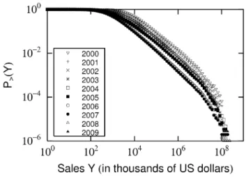
Figure 2: Distributions of sales Y for Japanese firms in 2000 to 2009. The number of firms changes across years but on average is 399,982.
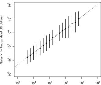
Figure 3: Relationship between tangible fixed assets K and sales Y for Japanese firms in 2008. The horizontal axis shows the values of K for the tail part of its distribution (i.e., the range in which K follows a power-law distribution), while the vertical axis shows the values of Y . The dots and the bars represent, respectively, the mean and the standard deviation of log Y for each bin of K, which is of the same size in log. We fit a line, log Y = θKY log K + log aKY, to the dots, which is indicated by the dashed line.
Figs. 1 and 2 show the CDFs of K and Y for Japanese firms in various years. We see that the K and Y for each year have a power-law tail for values exceeding a certain size threshold. Next, we show that PJ(K, Y ) is invariant under the exchange of variables,
PJ(K, Y ) = PJ
õ Y aKY
¶1/θKY
, aKYKθKY
!
, (20)
which is denoted by Y ↔ aKYKθKY. Fig. 3 shows the relationship between K and Y for Japanese firms in 2008. The dashed line represents the line log Y = θKYlog K +log aKY with respect to which quasi-inversion symmetry holds. This line is estimated as follows.
Step 1: The range in which K follows a power-law distribution is identified by the method proposed by Ref. [40], which is a modified version of the method advocated by Ref. [41]. As shown in Figs. 1 and 2, the right-end part of each distribution decays quicker than the rest of the distribution due to the limited number of observations. Such a finite-size effect is not present in small datasets, so it is not regarded as important in Ref. [41]. However, in large datasets, such as the one used in this paper, distributions are seriously affected by the finite-size effect, so that a simple application of the method proposed by Ref. [41] could lead to a failure to correctly detect the range in which K follows a power-law distribution. To avoid this, Ref. [40] proposes to “thin out” observations before applying the procedure by Ref. [41]. We adopt this method to detect ¯K. We employ the same procedure for the distribution of Y to detect ¯Y .
Step 2: The power-law range of K is divided into bins which are of the same size in log, and the geometric average of Y is calculated for the observations belonging to each bin, which is shown by the round dots in Fig. 3. We then run a least squares regression to fit the line log Y = θKYlog K + log aKY
to the dots. A similar method was adopted in Refs. [18], [33]. Note that we apply the least squares method not to individual observations but to the dots so as to give an equal weight to the right and left ends of the distribution. Finally, we conduct a Kolmogorov-Smirnov test to confirm that (20) holds with respect to the estimated line.
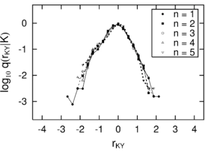
Next, let us consider the ratio between K and Y , which is denoted by RKY = Y /(aKYKθK Y). Fig. 4 shows the PDF of RKY conditional on K, which is denoted by Q(RKY | K). We see that the PDF of RKY does not depend on K, when K exceeds the size threshold ¯K. That is,
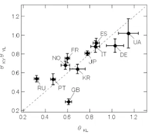
Q(RKY|K) = Q(RKY) for K > ¯K . (21) Finally, we check condition (17). We estimate μK/μY and θKY for twelve countries. The result is shown in Fig. 5. We fit a line to the data and obtain μK/(μYθKY) = 0.94 ± 0.03, indicating that the data are almost consistent with μK= θKYμY, although μK is slightly smaller than θKYμY.
Figure 4: PDFs of rKY(≡ log RKY) conditional on K. The range of K is divided into loga- rithmically equal size bins, which are given by K∈£104+0.2(n−1), 104+0.2n¢, n = 1, 2, · · · , 5.
Figure 5: Relationship between μK/μY and θKY in 2006 for twelve countries, namely Japan (JP, the number of observations is 723,109), France (FR, 887,142), Spain (ES, 718,729), Italy (IT, 611,988), Russian Federation (RU, 548,086), United Kingdom (GB, 342,370), Portugal (PT, 280,941), Korea (KR, 134,450), China (CN, 247,318), Ukraine (UA, 252,144), Norway (NO, 162,983) and Germany (DE, 213,017). The dashed line represents μK= θKYμY.
Figure 6: Relationship between θKL and θKYθY L for eleven countries in 2008. The dashed line represents θKL= θKYθY L.
4. Inversion Symmetry in Three-Dimensional Space
In the previous section, we observed inversion symmetry in the (log K, log Y ) plane and showed that inversion symmetry and Gibrat’s law lead to power laws for the distributions of K and Y . We apply the same analysis to the other sets of variables, that is (log Y, log L) and (log K, log L), to find that the three θ’s estimated by regressions (i.e., θKL, θKY, and θY L) are related to each other through θKL ' θKYθY L, as shown in Fig. 6. This result suggests the presence of inversion symmetry and Gibrat’s law in the three dimensional space (log K, log L, log Y ). In this section, we extend the discussion in Sec. 2 to three dimensional space.
Consider a plane in the three dimensional space (log u1, log u2, log v), which is given by
log v = θ1log u1+ θ2log u2+ log A, (22) and assume that the joint PDF of the three variables, PJ(u1, u2, v), is invertible in the sense that v↔ Au1θ1u2θ2. Specifically, inversion symmetry in the three dimensional space is defined as
PJ(u1, u2, v) = PJ
õ v
Au2θ2
¶1/θ1
,
µ v
Au1θ1
¶1/θ2
, Au1θ1u2θ2
!
. (23) We also assume a three-dimensional version of Gibrat’s law,
Q(R|u1, u2) = Q(R) for u1> ¯u1 and u2> ¯u2, (24) where ¯u1 and ¯u2 represent the size thresholds of u1 and u2, R is defined by R = v/(Au1θ1u2θ2), and Q(R|u1, u2) = PJ(u1, u2, R)/PJ(u1, u2). Note that R is closely related to what economists refer to as total factor productivity.
From (23) and (24), we obtain
PJ(u1, u2) = G(R)PJ(R1/θ1u1, R1/θ2u2), (25) which corresponds to (13) in Sec. 2. We expand (25) around R = 1 (namely, R = 1 + ² where ² ¿ 1) to obtain a differential equation. Under the assumption that u1 and u2are mutually independent, the solution to the differential equation is given by
PJ(u1, u2) = CTu1−μ1−1u2−μ2−1 , (26) where μ1and μ2 are positive parameters satisfying μ1θ+1
1 +
μ2+1
θ2 = G0(1). Note
that μ1 and μ2are the power-law exponents associated with u1and u2. Turning to the PDF of v, the result obtained by Refs. [35, 36] implies that, given the assumption that u1 and u2 are mutually independent, the product of u1 and u2 also follows a power-law distribution, with its exponent given by min{μ1/θ1, μ2/θ2}. Therefore, P (v) is given by
P (v)∝ v−μv−1 , (27)
where
μv= min{μ1/θ1, μ2/θ2} . (28) Note that (28) corresponds to (17) in the two dimensional case.
We now proceed to the empirical investigation of inversion symmetry in three dimensional space. We first eliminate the high correlation between log K and log L by converting (log K, log L) into (log Z1, log Z2). The new variables log Z1
and log Z2are defined as log Z1= √log L
2σlog L
+√log K 2σlog K
; log Z2= √log L 2σlog L −
log K
√2σlog K
, (29)
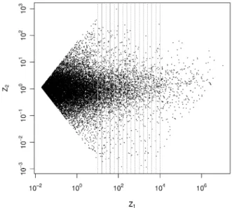
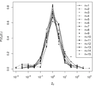
where σlog K and σlog L are the standard deviations of log K and log L, respec- tively. We have confirmed that Z1 and Z2 follow power-law distributions for Z1 > ¯Z1 and Z2 > ¯Z2. Note that, by construction, log Z1 and log Z2 are uncorrelated, but this does not necessarily imply that they are mutually inde- pendent. To see whether they are mutually independent or not, we conduct a Kolmogorov-Smirnov test as follows. We first divide the range of Z1into 15 bins of logarithmically equal size, which are given by Z1 ∈ [101+0.2(n−1), 101+0.2n) for n = 1, . . . , 15, as illustrated in Fig. 7. The distributions of Z2 conditional on Z1, that is, P (Z2 | Z1 ∈ [101+0.2(n−1), 101+0.2n)), are shown in Fig. 8. The figure shows that the PDFs for different values of n are almost identical, which is confirmed by the Kolmogorov-Smirnov tests indicating that the null hypoth- esis that, for any pair of the 15 distributions, the two distributions are identical cannot be rejected at the 5 percent significance level.
We then fit a plane, log Y = θZ1Y log Z1+ θZ2Ylog Z2+ log A, to the ob- servations for Z1 > ¯Z1 and Z2 > ¯Z2 to obtain estimates for θZ1Y and θZ2Y. For Japanese firms in 2008, the estimate of θZ1Y turns out to be 0.38 with a standard error of 0.005, while the estimate of θZ2Y is 0.08 with a standard error
Figure 7: Scatter plot of Z1 and Z2 for firms with K > ¯K and L > ¯L. The plot are for Japanese firms in 2008. The thin vertical lines indicate the bins of Z1, which are given by Z1∈ [101+0.2(n−1), 101+0.2n) for n = 1, . . . , 15.
Figure 8: PDFs of Z2 conditional on Z1, which are given by P (Z2 | Z1 ∈ [101+0.2(n−1), 101+0.2n)) for n = 1, . . . , 15.
of 0.01. We have confirmed the presence of inversion symmetry with respect to this estimated line (i.e., Y ↔ AZ1θZ1YZ2θZ2Y) as well as the presence of Gibrat’s law.
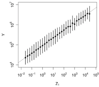
Next, we check whether condition (28) holds in the data. For Japanese firms in 2008, the estimate of the power-law exponent associated with Z1, which is denoted by μZ1, is 0.38 with a standard error of 0.01, while the es- timate of the power-law exponent for Z2, denoted by μZ2, is 1.16 with a stan- dard error of 0.01. Therefore, μZ1/θZ1Y is 0.99 and μZ2/θZ2Y is 14.5, so that min{μZ1/θZ1Y, μZ2/θZ2Y} = 0.99 ± 0.03. In other words, the theoretical pre- diction is that the power-law exponent associated with Y should be 0.99. In fact, the estimate of the power-law exponent for Y turns out to be 0.95 with a standard error of 0.01, which is close to the theoretical prediction. Furthermore, we find inversion symmetry between log Z1 and log Y in two dimensional space, as shown in Fig. 9. It is important to note that the slope of the fitted line in Fig. 9 is 0.38 ± 0.003, which is quite close to the estimate of θZ1Y obtained in three dimensional space. We also confirm the presence of Gibrat’s law in the (log Z1, log Y ) space, as shown in Fig. 10. These two results indicate that the presence of inversion symmetry and Gibrat’s law in two dimensional space is just a reflection of inversion symmetry and Gibrat’s law in three dimensional space, as predicted by the theoretical considerations above.
The inversion symmetry in three dimensional space discussed in this section also has a meaning in terms of economics. To show this, we first note that inversion symmetry in the (log Z1, log Z2, log Y ) space can be converted into inversion symmetry in the (log K, log L, log Y ) space, with the axis of inversion symmetry given by
log Y = α log K + β log L + log A , (30) where α and β are defined by
α = θZ√1Y − θZ2Y 2σlog K
; β = θZ√1Y + θZ2Y 2σlog L
. (31)
We denote this inversion symmetry by Y ↔ AKαLβ. Eq. (30) is referred to as the Cobb-Douglas production function by economists and has been widely used in economics since it was first introduced in 1928 by Ref. [37]. Specifi- cally, economists have been using the idea of production functions to describe the nonlinear relationship between output and inputs. At the firm-level, for example, the output of a firm, Y (e.g., measured in terms of sales), is a positive function of, e.g., the number of people working for the firm, L, and the number of machines it uses, K, as well as the productivity of the firm, A that is, the efficiency with which these inputs are used. This relationship is referred to as a production function, and the most widely used functional form for production functions is the Cobb-Douglas form. Although there are a number of studies by economists, such as [42]—[44], seeking to provide a theoretical foundation for the Cobb-Douglas functional form, no consensus has yet been found. The discus- sion in this section provides a new theoretical foundation for the Cobb-Douglas form.
Figure 9: Relationship between Z1and Y for Japanese firms in 2008. The dots and the bars represent, respectively, the mean and the standard deviation of log Y for each bin of Z1, which is of the same size in log. We fit a line, log Y = θZ1Ylog Z1+ log a1, to the data, which is indicated by the dashed line.
Figure 10: PDFs of r1 conditional on Z1, where r1 is defined as r1 ≡ log[Y/(a1Z1θZ1Y)]. The range of Z1 is divided into bins of the same size in log, which are given by Z1 ∈
£100.5(n−1), 100.5n¢, n = 1, 2, · · · , 5.
5. Conclusion
In this paper, we discussed the mechanism through which inversion sym- metry and Gibrat’s law generate power-law distributions with different tail ex- ponents. Using a dataset containing firm size variables for firms in various countries, that is, tangible fixed assets K, the number of workers L, and sales Y , we confirmed that they have power-law tails with different exponents. We also confirmed that inversion symmetry and Gibrat’s law hold, and that the power law exponents for K, L, and Y satisfy the relationship implied by theory. Based on these findings, we argue that there exists a plane in the three di- mensional space (log K, log L, log Y ), with respect to which the joint probability density function for the three variables is invariant under the exchange of vari- ables. We provide empirical evidence that this plane fits the data well and argue that the plane can be interpreted as the Cobb-Douglas production function, a type of function which has been extensively used in various areas of economics. In this sense, this paper provides a theoretical foundation for the Cobb-Douglas functional form.
The analysis in this paper provides suggestions for new avenues of research on Cobb-Douglas production functions. As mentioned, the Cobb-Douglas form is given by Y = AKαLβ, where A represents the level of productivity of a firm, and α and β are positive parameters. The first avenue for further research concerns the values of α and β. In economics, it is important to know whether the sum of these two parameters equals unity or not. For example, Ref. [45] found that the sum of the two is close to unity in some countries but less than unity in others. The second potential research avenue concerns where the tail exponent of Y comes from. The Cobb-Douglas form shown above implies that it should come from the exponent of K, the exponent of L, or the exponent of A. Business persons often argue that the key to achieving high sales growth is high productivity growth, implying that the upper tail of Y should stem from the upper tail of A. However, Ref. [46] has shown that the power-law exponent of the productivity distribution in a country tends to be greater than the power law exponent of the sales distribution in that country, indicating that the upper tail of the productivity distribution is less heavy than that of the sales distribution. In a related context, Refs. [47, 48] examined the distribution of labour productivity for Japanese firms. Investigating in more detail how the fat tail of sales distributions is related to the tails of the distributions of productivity and other firm variables is a task we hope to address in the future.
Acknowledgement
This study was supported in part by a Grant-in-Aid for Scientific Research (C) (No.20510147) and a Grant-in-Aid for Creative Scientific Research (No.18GS0101) from the Ministry of Education, Culture, Sports, Science and Technology, Japan.
References
[1] H. E. Stanley, Introduction to Phase Transitions and Critical Phenomena, Clarendon Press, Oxford, 1971.
[2] V. Pareto, Cours d’´Economie Politique, Macmillan, London, 1897. [3] M. E. J. Newman, Contemporary Physics 46 (2005) 323-351.
[4] A. Clauset, C. R. Shalizi, M. E. J. Newman, SIAM Review 51 (2009) 661- 703.
[5] E. Bonabeau, L. Dagorn, Phys. Rev. E 51 (1995) R5220. [6] S. Render, Eur. Phys. J. B 4 (1998) 131-134.
[7] M. Takayasu, H. Takayasu, T. Sato, Physica A 233 (1996) 824-834. [8] A. Saichev, Y. Malevergne, D. Sornette, Theory of Zipf’s Law and Beyond,
Springer, 2009.
[9] T. Kaizoji, Physica A 326 (2003) 256-264. [10] T. Yamano, Eur. Phys. J. B 38 (2004), 665-669. [11] A. Ishikawa, Physica A 371 (2006) 525-535.
[12] A. Ishikawa, Prog. Theor. Phys. Supple. 179 (2009) 103-113. [13] R. N. Mantegna, H. E. Stanley, Nature 376 (1995) 46-49. [14] R. L. Axtell, Science 293 (2001) 1818-1820.
[15] B. Podobnik, D. Horvatic, A. M. Petersen, B. Uro˘sevi´c, H. E. Stanley, Proc. Natl. Acad. Sci. 107 (2010) 18325-18330.
[16] D. Fu, F. Pammolli, S. V. Buldyrev, M. Riccaboni, K. Matia, K. Yamasaki, H. E. Stanley, Proc. Natl. Acad. Sci. 102 (2005) 18801-18806.
[17] B. Podobnik, D. Horvatic, F. Pammolli, F. Wang, H. E. Stanley, I. Grosse, Phys. Rev. E 77 (2008) 056102.
[18] K. Okuyama, M. Takayasu, H. Takayasu, Physica A 269 (1999) 125-131. [19] J. J. Ramsden, G. Kiss-Hayp´al, Physica A 277 (2000) 220-227.
[20] T. Mizuno, M. Katori, H. Takayasu, M. Takayasu, Empirical Science of Financial Fluctuations, Springer Verlag Tokyo (2002) 321-330.
[21] E. Gaffeo, M. Gallegati, A. Palestrinib, Physica A 324 (2003) 117-123. [22] J. Zhang, Q. Chen, Y. Wang, Physica A 388 (2009) 2020-2024. [23] H. Kesten, Acta Math. 131 (1973) 207-248.
[24] M. Levy, S. Solomon, Int. J. Mod. Phys. C 7 (1996) 595-601. [25] D. Sornette, R. Cont, J. Phys. I 7 (1997) 431-444.
[26] H. Takayasu, A. Sato, M. Takayasu, Phys. Rev. Lett. 79 (1997) 966-969. [27] Y. Fujiwara, W. Souma, H. Aoyama, T. Kaizoji, M. Aoki, Physica A 321
(2003) 598-604
[28] Y. Fujiwara, C.D. Guilmi, H. Aoyama, M. Gallegati, W. Souma, Physica A 335 (2004) 197-216.
[29] R. Gibrat, Les In´egalit´es ´Economiques, Sirey, Paris, 1932. [30] J. Sutton, J. Econ. Lit. 35 (1997) 40-59.
[31] M. Tomoyose, S. Fujimoto, A. Ishikawa, Prog. Theor. Phys. Supple. 179 (2009) 114-122.
[32] G. Bottazzi, Physica A 388 (2009) 1133-1136.
[33] H. Watanabe, H. Takayasu, M. Takayasu, Statistical Studies on Interrela- tionships of Financial Indicators of Japanese Firms, The Physical Society of Japan 2009 Autumn Meeting, in Japanese.
[34] C. K¨uhnert, D. Helbing, G. B. West, Physica A 363 (2006) 96-103. [35] A. H. Jessen, T. Mikosch, Inst. Math. 94 (2006) 171-192.
[36] X. Gabaix, Annu. Rev. Econ. 1 (2009) 255-293.
[37] C. W. Cobb, P. H. Douglas, Amer. Econ. Rev. 18 (1928) 139-165.
[38] H. Aoyama, Y. Fujiwara, M. Gallegati, Micro-Macro Relation of Pro- duction: The Double Scaling Law for Statistical Physics of Economy, arXiv:1003.2321v1.
[39] Bureau van Dijk, http://www.bvdinfo.com/Home.aspx.
[40] S. Fujimoto, A. Ishikawa, T. Mizuno, T. Watanabe, Economics E-Journal 5 (2011) 2011-20.
[41] Y. Malevergne, V. Pisarenko, D. Sornette, Phys. Rev. E 83 (2011) 036111. [42] H. S. Houthakker, Review of Economics Studies 23 (1955) 27-31.
[43] S. Rosen, Economica 45 (1978) 235-250.
[44] C. I. Jones, Quarterly Journal of Economics 120 (2005) 517-549.
[45] T. Watanabe, T. Mizuno, A. Ishikawa, S. Fujimoto, Economic Review (Keizai Kenkyuu) 62 (2011) 193-208.
[46] T. Mizuno, T. Watanabe, A. Ishikawa, S. Fujimoto, Prog. Theor. Phys. Supple. 194 (2012) 122-134.
[47] W. Souma, Y. Ikeda, H. Iyetomi, Y. Fujiwara, Economics E-Journal 3 (2009) 2009-14.
[48] Y. Ikeda, W. Souma, Prog. Theor. Phys. Supple. 179 (2009) 93-102.
![Figure 10: PDFs of r 1 conditional on Z 1 , where r 1 is defined as r 1 ≡ log[Y/(a 1 Z 1 θ Z1Y )].](https://thumb-ap.123doks.com/thumbv2/123deta/5651078.6494/16.892.254.627.420.750/figure-pdfs-conditional-z-defined-log-y-z.webp)
