SIMULTANEOUS ESTIMATION OF DYNAMIC ORIGIN-DESTINATION (O-D) TRAVEL TIME AND FLOW USING NEURAL-KALMAN FILTER TECHNIQUE
WITH THE MACROSCOPIC TRAFFIC FLOW SIMULATION MODEL
by
Hironori Suzuki
A dissertation submitted in partial fulfillment of the requirements for the degree of Doctor of Engineering.
Examination Committee Dr. Kiyoshi Takahashi (Chairman) Prof. Yordphol Tanaboriboon Dr. Pannapa Herabat
Prof. Vilas Wuwongse Dr. Takashi Nakatsuji
External Examiner Prof. Nagui M. Rouphail, Ph.D. School of Civil Engineering, North Carolina State University
Nationality Japanese
Previous Degree(s) Master of Engineering
Department of Transportation Engineering Graduate School of Science and Technology Nihon University
Tokyo, Japan
Bachelor of Engineering
Department of Transportation Engineering School of Science and Technology
Nihon University Tokyo, Japan
Scholarship Donor Government of Japan
Asian Institute of Technology School of Civil Engineering
Bangkok, Thailand April 2001
ACKNOWLEDGEMENT
This dissertation could not have been completed without cooperation from many people. First of all, the author wishes his sincere appreciation and heartfelt acknowledgment to his former advisor, Dr. Takashi Nakatsuji who has spent a lot of valuable time and expenses for completing this dissertation and gave valuable chances for writing journal papers and presenting parts of dissertation works at international conferences. His kindness, appropriate assistance, frequent and worthy discussions for the dissertation work are very much appreciated.
The author also wishes his heartfelt appreciation to Dr. Atsushi Fukuda, an associate professor of Nihon University who encouraged the author to be interested in traffic problems in Asian countries, and gave a chance to study at AIT. He has taught the general procedure of writing scientific papers; how to find and tackle the existing problems, how to write papers and how to make a good presentation at conferences.
The author would also like to extend his sincere thanks to Dr. Kiyoshi Takahashi for his support and supervision as an official advisor. He also spent his precious time for supervising and completing this dissertation works. His kindness and guidance were admired when the authors faced various problems in completing this dissertation works.
The author also wishes to express honest thanks to Transportation and Infrastructure Engineering Program coordinator and a member of his committee, Prof. Yordphol Tanaboriboon for his guidance and support during his stay at AIT. He really made the life at AIT enjoyable and memorable one. Without his assistance, the life in Thailand would have been worthless.
The author would also like to express thankfulness to Dr. Pannapa Herabat and Prof. Vilas Wuwongse for granting precious time to be parts of the examination committee, and suggesting the author to write papers for international conferences.
The author wishes his sincere appreciation to Prof. Nagui M. Rouphail, a professor of North Carolina State University for evaluating this dissertation as his external examiner. He granted many valuable comments and recommendations to bring this dissertation up to internationally acceptable one. Revision work based on his comments and recommendations was all taken into this dissertation.
The author would also like to express his lots of thanks to Mr. Gemunu S. Gurusinghe, a senior lecturer of the University of Peradeniya for taking care of the author as his father, friend and teacher. He granted lots of his precious time for teaching English and the life in an international society. We shared most of our time during the life at AIT, and the author could learn various things through the life with him. This dissertation works could not have been completed without his sincere guidance and assistance.
The author is also grateful to Mr. Terry Clayton for checking and correcting English in this doctoral dissertation. Also, he always accepted his kind requests for checking his English in many journal papers for the publication.
The author is indebted to his colleagues who supported his field data collection especially Mr. Nobutaka Yamamoto, Mr. Sakda Penwai and Mr. Vichapat Pataravuth. The author would also like to thank all his classmates and friends for their help, moral support and encouragement throughout his stay at AIT.
The author utterly desires to express his special appreciation to his ever-loving wife Kumiko for her kindness and warmness that brought him to this stage.
Finally, this dissertation is dedicated to the author’s beloved parents and ever-loving older brother.
ABSTRACT
A new model was formulated for estimating dynamic origin-destination (O-D) travel time and flow on a long freeway using a Neural-Kalman filter, which was originally developed by the authors. The model predicts O-D travel times and flows simultaneously by using traffic detector data such as link traffic volumes, spot speeds and off-ramp volumes. The model is based on a Kalman filter that consists of two equations; state and measurement equations. First of all, the state and measurement equations of the Kalman filter were modified to consider the influence of traffic states for some previous time steps. Then, artificial neural network (ANN) models were integrated with the Kalman filter to enable non-linear formulations of the state and measurement equations. Finally, a macroscopic traffic flow simulation model was introduced to simulate traffic states on a freeway in advance and predict traffic variables such as O-D travel times, link traffic volumes, spot speeds and off- ramp volumes. The new model was compared with a Regression-Kalman filter in which the state and measurement equations are defined by regression models. The numerical analysis showed that the new model was capable of estimating non-linearity of dynamic O-D travel time and flow and helped to improve their estimation precision under free flow traffic states as well as congested flow states. The estimation precision was improved if dynamic O-D travel time and flow were simultaneously estimated within one process. In addition, another numerical analysis revealed that the use of more number of traffic detectors contributed to estimating the O-D travel time and flow with more accuracy.
TABLE OF CONTENTS
Chapter Title Page
Title Page i
Acknowledgment ii
Abstract iii
Table of Contents iv
List of Figures vii
List of Tables viii
1. Introduction 1
1.1 General Background 1
1.2 Problem Statement 3
1.3 Purpose and Objectives 3
1.4 Organization of the Dissertation 4
2. Literature Survey 6
2.1 O-D Flow Estimation 6
2.1.1 Static Approach 6
2.1.2 Dynamic Approach 7
2.2 Travel Time Estimation 15
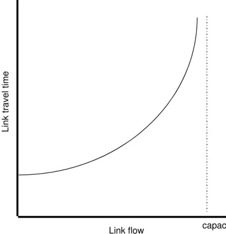
2.2.1 Link Travel Time Estimation 17
2.2.2 Characteristics of Travel Time 18
2.2.3 O-D Travel Time Estimation 19
2.3 Relationship between O-D Travel Time and Flow 23
2.4 Kalman Filter 23
2.4.1 Theory 24
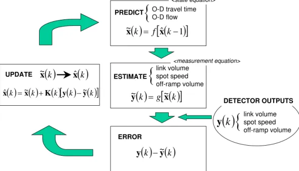
2.4.2 General Estimation Algorithm by a Kalman filter 35 2.4.3 Application of Kalman Filter for Estimating Traffic States 36
2.5. Artificial Neural Network (ANN) Model 37
2.6 Macroscopic Traffic Flow Simulation Model 40
2.6.1 Modeling 40
2.6.2 Parameter Estimation by the Box’s Complex Algorithm 45
2.6.3 Validation of macroscopic model 48
2.7 Summary 49
3. Model Development 51
3.1 Feedback Estimation by Kalman Filter 51
3.2 Definition of O-D travel time and flow 53
3.2.1 O-D Flow 53
3.2.2 O-D Travel Time 55
3.2 Modification of an Extended Kalman Filter 55
3.2.1 State Equation 56
TABLE OF CONTENTS (CONTINUED)
Chapter Title Page
3.2.2 Measurement Equation 58
3.2.3 Modification of Extended Kalman Filter 60
3.3 Neural-Kalman Filter 63
3.3.1 Neural-Kalman Filter (NKF) 63
3.3.2 Regression Kalman Filter (RKF) 67
3.4 Macroscopic Traffic Flow Model 68
3.5 Procedure of O-D Travel Time and Flow Estimations using a NKF 71
3.5.1 Basic Procedure 71
3.5.2 Introduction of a Macroscopic Model 72
3.6 Summary 74
4. Data Collection 75
4.1 Field Data Collection 75
4.1.1 Study Area 75
4.1.2 Allocation of Surveyors 81
4.1.3 Procedure and Equipment 85
4.1.4 Measurement Data 86
4.2 Simulated Traffic Data by FRESIM 87
4.2.1 Outline of FRESIM 87
4.2.2 Calibration of the FRESIM model for the FES and SES 89
4.2.3 Validation 92
4.3 Data Processing 95
4.3.1 Link Traffic Volume and Spot Speed 96
4.3.2 O-D Travel Time 97
4.3.3 O-D Flow 98
4.4 Summary 99
5. Numerical Analyses 100
5.1 Study Area 100
5.2 Evaluation Procedures 102
5.2.1 Step 1 (RKF without Advance Prediction of Traffic States) 102 5.2.2 Step 2 (NKF without Advance Prediction of Traffic States) 102
5.2.3 Step 3 (NKF with macroscopic model) 102
5.3 ANN models 103
5.3.1 ANN Model for State Equation 103
5.3.2 ANN Model for Measurement Equation 104
5.4 Parameter Estimation of a Macroscopic Model 105
5.5 Scenario 106
5.5.1 Free Flow States (Case 1) 106
5.5.2 Congested Flow States (Case 2) 108
5.6 Experimental Results 109
5.6.1 Free Flow States 109
TABLE OF CONTENTS (CONTINUED)
Chapter Title Page
5.6.2 Congested Flow States (Case 2) 114
5.7 Discussion of the Results 118
5.7.1 Effect of ANN Models 118
5.7.2 Effect of predicting traffic states 119
5.8 Effect of Simultaneous Estimations 119
5.8.1 Procedure 120
5.8.2 Experimental Results 120
5.9 Summary 124
6. Effect of the Number of Measurement Points 126
6.1 Traffic Data 126
6.2 ANN models 129
6.3 Calibration and Validation 129
6.4 Procedure 130
6.5 Experimental Results 131
6.5.1 “Light” Condition 131
6.5.2 “Heavy” Condition 134
6.6 Discussion 137
6.7 Summary 138
7. Conclusion and Recommendation 139
7.1 Conclusion 139
7.2 Recommendations 140
7.2.1 Recommendation for Neural-Kalman Filter 131 7.2.2 Another Approach for O-D Travel Time and Flow Estimations 134
References 143
Appendix 151
LIST OF FIGURES
Figure No. Title Page
2.1 Conventional link travel time function 17
2.2 Travel time under congested flow states 18
2.3 Actual O-D travel time by summing up link travel times 20
2.4 Feedback O-D travel time estimation model 22
2.5 A Feedback estimation algorithm by a Kalman filter 36
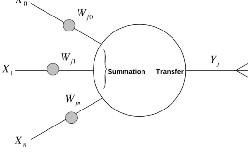
2.6 A neuron 37
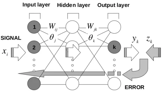
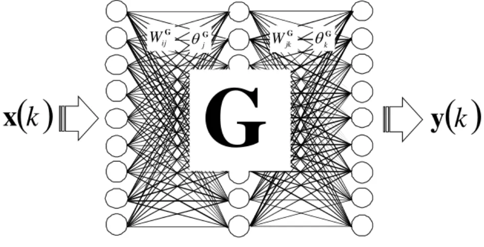
2.7 ANN model with three layers 38
2.8 Traffic flow conservation 42
2.9 Box’s complex algorithm logic diagram 47
3.1 Feedback process by Kalman filter 52
3.2 A freeway corridor 54
3.3 ANN model for state equation 66
3.4 ANN model for measurement equation 66
3.5 Lane closure type 1 70
3.6 Lane closure type 2 70
3.7 Procedure of NKF 73
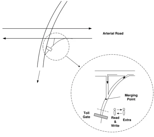
4.1 Study area 76
4.2 Geometry at HP 78
4.3 Geometry at EP 78
4.4 Geometry at SSP 79
4.5 Allocation of surveyors 81
4.6 Geometry of TU, CW and RP 82
4.7 Geometry of NW 83
4.8 Geometry of SV and RM 83
4.9 Geometry of SV62 84
4.10 Geometry of BN 84
4.11 Check points for floating car survey 86
4.12 FRESIM model for the FES and SES 91
4.13 Comparison of actual vs. FRESIM flow and speed (HP) 92 4.14 Comparison of actual vs. FRESIM flow and speed (EP) 93 4.15 Comparison of actual vs. FRESIM flow and speed (SSP) 93 4.16 Comparison of Root Mean Square Errors (RMSEs) 94 4.17 Comparison of actual vs. FRESIM O-D travel time (CW-BN) 95
4.18 Example of FRESIM output (Link statistics) 96
4.19 An Example of FRESIM output (spot speed) 97
4.20 Calculation of O-D travel time by summing up link travel times 98
4.21 An example of origin-destination trip table 99
5.1 A freeway corridor 101
5.2 Estimation procedure 103
LIST OF FIGURES (CONTINUED)
Figure No. Title Page
5.3 ANN model for state equation 104
5.4 ANN model for measurement equation 104
5.5 Artificial data generation 107
5.6 Comparison of O-D travel times (RKF vs. NKF) 110 5.7 Comparison of O-D travel times
(NKFs with vs. without advance prediction) 110
5.8 Comparison of O-D flows (RKF vs. NKF) 111
5.9 Comparison of O-D flows
(NKFs with vs. without prediction of traffic states) 112
5.10 RMS errors of O-D travel time estimations 113
5.11 RMS errors of O-D flow estimations 113
5.12 Comparison of O-D travel times (RKF vs. NKF) 114 5.13 Comparison of O-D travel times
(NKFs with vs. without prediction of traffic states) 115
5.14 Comparison of O-D flows (RKF vs. NKF) 116
5.15 Comparison of O-D flows
(NKFs with vs. without prediction of traffic states) 116 5.16 RMS errors of O-D travel time estimations (Congested flow states) 117 5.17 RMS errors of O-D flow estimations (Congested flow states) 118 5.18 Separate and simultaneous estimates of O-D travel time (NW-BN) 121 5.19 RMS Errors of separate and simultaneous estimations of
O-D travel time 121
5.20 Separate and simultaneous estimates of O-D flow (NW-BN) 122 5.21 RMS Errors of separate and simultaneous estimations of O-D Flow 123
6.1 A Freeway model 127
6.2 Inflow volumes of each data pattern 128
6.3 Change of diverging rates at D1 and D2 128
6.4 ANN model for state equation 129
6.5 ANN model for measurement equation 129
6.6 Comparison of O-D travel time estimates (“Light” condition) 132 6.7 Comparison of O-D flow estimates (“Light” condition) 132 6.8 RMS errors of O-D travel time estimations (“Light” condition) 133 6.9 RMS errors of O-D flow estimations (“Light” condition) 133 6.10 Comparison of O-D travel time estimates (“Heavy” condition) 135 6.11 Comparison of O-D flow estimates (“Heavy” condition) 135 6.12 RMS errors of O-D travel time estimations (“Heavy” condition) 136 6.13 RMS errors of O-D flow estimations (“Heavy” condition) 136
LIST OF TABLES
Table No. Title Page
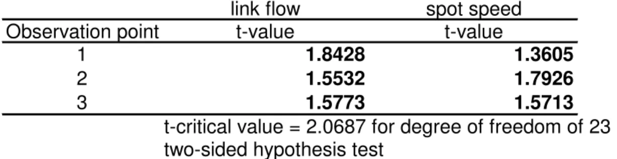
4.1 Results of t-test for link traffic volumes and spot speeds 94
5.1 Optimized macroscopic parameters 105
5.2 T-test for validating macroscopic model 106
5.3 The number of data sets for training ANN models 107 5.4 Calibration and validation data sets (free flow states) 108 5.5 Calibration and validation data sets (congested flow states) 109
6.1 The Number of synapse weights and data sets 130
6.2 Three sets of measurement points 130
CHAPTER I
INTRODUCTION
1.1 General Background
Various techniques of Intelligent Transport Systems (ITS) will contribute to providing real time traffic information on traffic congestion, incidents, travel time and so on. Dynamic information will allow drivers to select appropriate routes and/or departure times to avoid congestion and minimize travel time. Origin-destination (O-D) travel time is the most important factor for route choice and departure time selection behaviors (Khattak et al., 1996), and should be updated incessantly to provide more accurate information for drivers to make decisions frequently (Abdel-Aty et al., 1995). Also, dynamic O-D flow information is prerequisite for traffic administrators, who are in charge of managing toll gates on freeway networks. This management would alleviate queuing and waiting time at off-ramps, and help to prevent queuing vehicles from overflowing onto the main lines of freeways.
For the last two decades, numerous studies have been made for estimating O-D travel time or flow on freeways and urban road networks. Early studies on O-D flow estimations were done as static approaches established mainly in the transportation planning field. The static approach is a technique to estimate them among widely distributed origin and destination zones over a long time period (e.g. one hour or one day). There have been many models proposed such as gravity type models (Nihan, 1982; Stokes and Morris, 1984), entropy maximizing and information minimizing approach (Van Zuylen and Willumsen, 1980), Bayesian approach (Maher, 1983) and least square method (Hendrickson and McNeil, 1984). However, they require additional “a priori” information such as target O-D trip matrix. Since it is extremely difficult to obtain such information for a short time period, they are not applicable for dynamic problems.
Studies on the dynamic estimations of O-D travel time and flow can be broadly classified into two approaches. One is a feed-forward approach based on drivers’ behavior models which attempt to estimate them according to the behavior of each driver under certain traffic conditions. Travel simulators have been used to create hypothetical experimental data for modeling as well as analyzing drivers’ behavior. In spite of extensive efforts, the driving simulators are still not successful in representing realistic driving environments and conditions (Koutsopoulos et al., 1995).
The other is a feedback approach based on measurement data, taking into account how dynamic changes in O-D travel time or flow can be reflected in real-time traffic data on link traffic volumes, spot speeds and so on. The O-D travel time or flow are estimated indirectly from the traffic data at some measurement points. Once the detectors measure any changes in the traffic conditions, the feedback model can immediately reflect the changes in the estimates of dynamic O-D travel time and flow. As Ben-Akiva et al. (1991) pointed out in their study, travel time information should be estimated with accuracy and updated frequently because
drivers’ expected travel times are always changing according to dynamic traffic conditions. A Kalman filter is a suitable method for estimating dynamic O-D travel time because it gives the estimates in real time by measuring the dynamic changes of traffic states.
In general, a Kalman filter consists of two equations, state and measurement equations. The state equation used to describe the time-series changes of state variables such as O-D travel time and flow, whereas the measurement equation defines the relationship between the state variables and measurement data such as link traffic volumes and spot speeds. Both equations are generally described in analytical equations.
Cremer and Keller (1981) tackled an O-D flow estimation problem at a large complicated intersection. Later, they formulated the problem using a Kalman filter model (1987), an Ordinary Least Squares (OLS) approach and a Constant OLS method (1984). Bell (1989) developed a time-dependent O-D matrix estimation model for a small road network based on the approach by Cremer and Keller (1987). The above models, however, are limited to a large isolated intersection or a small road network.
Ashok and Ben-Akiva (1993) applied a Kalman filter for estimating O-D flows from link traffic counts on a long freeway. The model requires a lot of effort to compute coefficient matrices of the measurement equation, and assumes that travel times are constant over the estimation time period. This assumption made the model unsuitable for an actual implementation on a long freeway. Chang and Wu (1994) considered dynamic travel time for estimations of O-D flows on a freeway corridor using a Kalman filter. They assumed that link traffic volumes at measurement points were influenced by O-D flows departed their origins several time steps before. The time step was calculated from the average travel time taken by vehicles to traverse between origins and measurement points. In order to reduce the number of parameters in the Kalman filter formulation, however, they considered the O-D flows only at two previous points and neglected most of other influential O-D flows. Travel time was not fully taken into account for dynamic O-D flow estimations. Another Kalman filter approach was proposed by Madant et al. (1996), which considered dynamic change in travel time. However, it has no feedback from the O-D flow to O-D travel time because a traffic simulator independently calculates the O-D travel time. Many models are not applicable for estimating both O-D travel time and flow simultaneously in one process even though they are strongly correlated with each other. In addition, travel times are solely implicit variables in any O-D flow estimation models.
Wong and Sussman (1973), Fu and Rilett (1995) attempted to estimate dynamic O-D travel time indirectly from departure times and the coordinates of origins and destinations. However, they did not succeed in estimating real-time O-D travel time because it is not solely the function of the departure time and the coordinates only. Nakatsuji et al. (1997) first tackled a dynamic O-D travel time estimation on a long freeway using a Kalman filter. For more precise estimation, the coefficient matrices of the state and measurement equations were updated when measuring on-line detector data and actual O-D travel time aggregated at off- ramps every time step. However, there was a significant time lag until drivers exit the freeway at off-ramps because they drive quite long distance. It takes a long time for the actual O-D travel time measured at off-ramps to be taken up to dynamic estimates of drivers’ expected O-D travel time at on-ramps. The time lag brought large errors in estimating O-D
coefficient matrices because they adopted linear regression models for defining the state and measurement equations.
1.2 Problem Statement
As demonstrated in the literatures, a Kalman filter approach has the potential for estimating O-D travel time or flow on freeways and urban road networks, particularly where traffic detectors are densely installed. However, some problems need to be addressed before it is applied to a long freeway and a large urban road network.
First, the interactions among O-D travel time, flow and some measurement variables are very complicated when a Kalman filter is applied to a long freeway. The interactions are generally non-linear and almost impossible to describe in analytical form. This makes definitions of the state and measurement equations and derivation of the coefficient matrices quite difficult tasks. It is preferable to define both equations in non-linear formulae rather than linear regression models.
Secondly, a Kalman filter would create large errors when estimating O-D travel time on a long freeway. The errors were caused by the significant time lag until the measured O-D travel time at off-ramp is reflected in dynamic estimates of drivers’ expected O-D travel time at on-ramps. An advance prediction of traffic states would help to alleviate the time lag and afford more accurate estimates of O-D travel time.
Thirdly, there are few models for estimating O-D travel time and flow simultaneously in one process although they are strongly correlated with each other. If a freeway is long, the effect of O-D travel time on O-D flow cannot be neglected. Also, O-D flow might be an important variable for estimating O-D travel time. The new model should consider the interaction between O-D travel time and flow, and estimate them simultaneously in one process for more accurate estimations.
Finally, a conventional Kalman filter considers the state variables for only one previous time step. On a long freeway, however, the current state variables are significantly influenced by those for several previous time steps. The Kalman filter should be theoretically expanded to fully take into account the state variables for as many influential previous time steps as possible.
1.3 Purpose and Objectives
This study aims to formulate a new model for the estimations of dynamic O-D travel time and flow on long freeways. The major objectives of this study are:
• To integrate artificial neural network (ANN) models with a Kalman filter to enable non- linear formulations of the state and measurement equations. ANN models make it possible to define the equations without assuming any analytical functions, and to describe complicated interactions among O-D travel time, flow and measurement variables.
• To introduce a macroscopic traffic flow model for predicting traffic conditions on a long freeway in advance. The advance prediction may avoid the significant time lag problem and reduce the errors in O-D travel time estimations on a long freeway.
• To estimate both O-D travel time and flow simultaneously in one process. Dynamic O-D travel time will be an important information for estimating O-D flow in real time, and vice versa.
• To generalize a Kalman filter for estimating both dynamic O-D travel time and flow on a long freeway. Both state and measurement equations are reformulated to take into account the influence of state variables for as many previous steps as possible.
• To investigate the effects of ANN models, the advance predictions of traffic conditions and the simultaneous estimations of O-D travel time and flow thorough numerical analyses.
In addition, this new method is featured as an indirect estimation method based on a feedback technique. It estimates O-D travel time and flow in real time while measuring traffic variables such as link traffic volumes, spot speeds and off-ramp volumes. It implies that the information given by traffic detectors have much possibility to estimate them more accurately. Hence, it is anticipated that the estimation precision will be improved by installing more number of traffic detectors. If traffic detectors are densely installed and are able to output reliable traffic data, a feed back estimation method may have the potential of providing the accurate estimates. Therefore, the influence of the number of detectors on estimation precision of O-D travel time and flow should be addressed in this study. This leads to a discussion how many detectors should be installed to satisfy the estimation precision required for an actual implementation of dynamic O-D travel time and flow estimations. Therefore, the last objective is:
• To analyze the influence of the number of detectors on the estimation precision of dynamic O-D travel time and flow. This is to show that the estimation precision partly depends on the number of detectors installed on freeways.
1.4 Organization of the Dissertation
This dissertation consists of seven chapters. A review of published literatures on static and dynamic O-D flow estimations, link travel time models, dynamic O-D travel time estimations, characteristic of travel time, is made in Chapter II. The theories of Kalman filter, ANN model and macroscopic model are also summarized. Dynamic models and feedback approaches are mainly covered in the literature survey.
Chapter III describes the formulation of a new proposed model for estimating dynamic O-D travel time and flow on long freeways. This chapter explains how to generalize the Kalman filter to be applicable to long freeways, how to integrate ANN models into the generalized Kalman filter and how to introduce a macroscopic model for the estimations. The procedure of the estimation using a new model is also given in this chapter.
Chapter IV focuses on data collections carried out on the expressways in Bangkok, Thailand on 22nd (Tuesday) and 23rd (Wednesday) December 1998. The procedure of the data collection and the aggregation are summarized together with the details of each survey point. In order to simulate traffic flows on extensive traffic situations, a microscopic freeway simulation model, FRESIM creates a virtual freeway network that imitates the expressways in Bangkok, and generates traffic data for numerical analyses. The FRESIM model is validated and the process of the traffic data is described.
Chapter V evaluates the new proposed model through numerical analyses. This chapter investigates how the ANN models and the advance prediction of traffic states are effective in providing more accurate estimates of O-D travel time and flow. The experimental results are shown along with some discussions. In addition, the effect of simultaneous estimations of O- D travel time and flow on their estimation precision is discussed.
The influence of the number of measurement points on the estimation precision is analyzed in Chapter VI. The methodology and results are described and discussed.
Chapter VII concludes the study and suggests further research in this study field.
CHAPTER II
LITERATURE SURVEY
This chapter aims to summarize studies on the estimations of O-D flow and travel time on freeway or urban road networks, and find out some problems in the current estimation models or techniques. This literature survey mainly focuses on the following three aspects: (1) O-D flow estimations, (2) travel time models and (3) brief theories of Kalman filter, artificial neural network model and a macroscopic model. The O-D flow estimations cover both static and dynamic approaches, even though the static methods are not the concern of this research. The review of travel time estimation techniques involves the estimations of link travel time, O-D travel time and the characteristics of travel time. Various techniques to estimate link travel time from traffic detector outputs are presented. Then, O-D travel times have been simply computed by summing up these link travel times along the O-D pairs. The studies on the travel time characteristics show how dynamic travel times are important for driver convenience. Since a new proposed model for estimating dynamic O-D travel time and flow involves three mathematical models such as a Kalman filter, an artificial neural network (ANN) model and a macroscopic model, their brief theories and applications are also summarized.
2.1 O-D Flow Estimation
Over the last two decades, O-D flow estimations have been a subject of controversy. This kind of study originally started in the transportation planning field, estimating static trip patterns between some origins and destinations for long time periods (e.g. ten or twenty years). Later, these studies were applied to dynamic O-D flow estimation problems for an isolated large intersection or small road networks. In recent years, some models have been proposed for the dynamic O-D flow estimations on a large freeway corridor.
2.1.1 Static Approach
Nihan (1982) and Stokes and Morris (1984) proposed gravity type models for static O-D flow estimation problems based on the Newton’s gravity low. Given the total number of entering and exiting volumes, each O-D flow can be determined according to the size of trip origin and destinations. Van Zuylen and Willumsen (1980) developed an entropy maximizing and information minimizing approach to estimate the most likely O-D flows using some link traffic volumes and any prior information about the O-D flows. Maher (1983) formulated a static O-D flow estimation model based on Bayesian approach. To determine a unique solution, prior beliefs about the O-D flows must be added. Hendrickson and McNeil (1984) proposed a least squares method. However, all static method requires additional “a priori” information such as target O-D flow matrix and so on. This research is limited to dynamic approaches only and does not deal with those static models.
2.1.2 Dynamic Approach
Cremer and Keller (1981) first tackled an O-D flow estimation problem for an isolated large intersection. They proposed a recursive method to estimate dynamic O-D travel time at a complicated intersection. Real-time traffic counts on entrance and exit volumes during time interval kyield recursive estimations of O-D flows. For describing the model, the following variables are introduced:
( )k
qi = inflow volume which enters entrance i during time interval k (i=1,2,,m)
( )k
yi = outflow volume which leaves exit j during time interval k (j=1,2,,n)
( )k
fij = O-D flow traveling from entrance i to exit j
( )k
bij = proportion of diverging volume at exit j entering at i
(
0≤bij ≤1)
Each exit volume yi( )k can be aggregated as the summation of all inflow volumes diverging at the exit j:
( ) ( ) ( )
k k kyi =q′ ⋅bj Eq. 2.1
where bj( )k is the ( )m*1 column vector of O-D flow proportions bij( )k ; and q′( )k is the ( )1*m
row vector of inflow volumes. Eq. 2.1 can be rewritten as vector and matrix form as follows:
( ) ( ) ( )
k q k B ky′ = ′ ⋅ Eq. 2.2
Here, y′( )k is the ( )1*n row vector of exit volumes, and B( )k is the (m *n) matrix of O-D flow proportions. Let ∆q′( )k and ∆yi( )k denote as the deviations of actual entrance and exit volumes from their mean values. The problem is to estimate O-D flow proportions bj( )k recursively by measuring actual volume deviations ∆q′( )k and ∆yi( )k . The recursive estimator is formulated as:
( )
k j( )
k( )
k[
yj( )
k yj( )
k]
j ˆ 1 ˆ
ˆ =b − + ⋅∆q ⋅ ∆ −∆
b γ Eq. 2.3
where, bˆi( )k is the estimates of bj( )k ; γ is a gain factor that has to be chosen appropriately (Cremer and Keller, 1997). The estimates of ∆yi( )k is given as:
( ) ( ) ( )
ˆ 1ˆ =∆ ′ ⋅ −
∆yj k q k bj k Eq. 2.4
Later, Cremer and Keller (1987) and Nihan and Davis (1987; 1989) proposed another recursive model based on a Kalman filter technique with the following state and measurement equations:
( )
k j( ) ( )
k kj b w
b +1 = + Eq. 2.5
and
( ) ( ) ( ) ( )
k k k v kyj =q′ ⋅bj + Eq. 2.6
The approaches by Cremer and Keller (1981; 1987) were developed only for an isolated large intersection. As shown in Eqs. 2.4 and 2.6, the O-D flow proportion matrix B( )k is divided into each column. This matrix decomposition is valid only when entrance and exit volumes are assumed to have no relationship among each entrance and exit. For a long freeway corridor, however, there may be complicated interactions among various traffic variables such as entrance, exit and link flow volumes and so on. This complication makes the Cremer and Keller’s model unsuitable for a long freeway.
Cremer and Keller (1984) also applied Ordinary Least Squares (OLS) and Constrained Ordinary Least Squares (COLS) for estimating real-time O-D flows at an intersection. These approaches were followed by Nihan and Davis (1987; 1989). For the OLS approach, it is assumed that the O-D flow proportion matrix B( )k is constant during time interval K. By recording the measurement data of ∆y′( )k and ∆q′( )k over time K, the following equation is formulated with the constant proportion matrix B:
( ) ( )
( )
( ) ( )
( )
B q
q q
y y y
⋅
∆ ′
∆ ′
∆ ′
=
∆ ′
∆ ′
∆ ′
K K
2 1 2
1
Eq. 2.7
Let Q and Yas: ( )( )
( )
∆ ′
∆ ′
∆ ′
= K q
q q
Q
2 1
and
( )( )
( )
∆ ′
∆ ′
∆ ′
= K y
y y
Y
2 1
, respectively.
Then, the estimates of O-D flow proportion matrix Bˆ can be computed as:
( ) ( )
QQ QYBˆ = ′ −1⋅ ′ Eq. 2.8
On the other hand, the COLS method provides the deterministic formula given in Eq. 2.9:
( ) ( )
q Byˆ′ k = ′k ⋅ ˆ Eq. 2.9
The solution of Eq. 2.9 can be obtained by solving the following optimization problem:
( ) ( )
y By ˆ
1 2
n ˆ mi
1 − → ′
=
∑
= K
k
k K k
J Eq. 2.10
The constraints for Eq. 2.10 are:
( ) (
k foralli j k)
bij 1 , ,
0≤ ≤ , b
( ) (
k foralli k)
n
j
ij 1 ,
1
∑
= = and bii( )
k =0(
fori=1,2,,min( )
m,n)
.These models require measuring traffic volumes entering and exiting the intersection at each time step, and keeping the dynamic data for some consecutive time steps to create the vectors,
Q and Y. However, these approaches have not succeeded in estimating real-time O-D flow proportion Bˆ because the consecutive time steps to be considered is very long for the actual dynamic implementations (e.g. forty minutes).
Bell (1991) proposed two models to estimate dynamic O-D flows, considering travel times on a small road network. The first model is based on the assumption that the travel time taken by a vehicle traveling between O-D pairs is geometrically distributed. The second one assumes that the fastest vehicle passes from any entrance to the specified exit within one time interval, whereas the slowest vehicle takes three time intervals. The second model is formulated as follows:
( )
t = 0( )
t + 1( )
t−1 + 2( )
t−2yj bj Tq bj Tq bj Tq Eq. 2.11
where, ( )t
yj = traffic volumes exiting a small road network at j during time interval t
( )t
qi = traffic volumes entering at i during time t
bijk = the proportion of inflow volumes at an origin i destined for exit at j with the travel time k
Similar to the studies by Cremer and Keller (1981; 1984), both models are formulated by an O-D flow proportion matrix divided into each column. In addition, the travel time to traverse the road networks is small enough to be neglected (Chang and Wu, 1994; Madanat et al., 1996). This is not a suitable assumption for dynamic O-D flow estimations on a long freeway.
Also, it should be noted that equations such as Eq. 2.1, 2.6 and 2.11 are sufficient for capturing the dynamic relationships between O-D patterns and exit volumes only if the traffic flow on the freeway is stable (Chang and Wu, 1994).
Ashok and Ben-Akiva (1993) formulated a model for estimating real-time O-D flows indirectly from link traffic volumes based on a Kalman filter technique. The model is formulated for an 180-mile freeway corridor. The deviations of O-D flows from the prior estimates are defined as state variables, whereas link traffic flows as measurement variables. The state equation is given as:
(
r p rHp)
rhh
q h p
n
r p r rh H
h r h
r x f x x w
x
OD − +
=
− ′ ′
− ′
= ′=
+ ′
+
∑ ∑
, ,1 1
, 1
, Eq. 2.12
where,
nOD = the number of O-D pairs
nl = the number of links equipped with vehicle detectors
xrh = the number of vehicles leaving origin during time interval h and travelling between the rth O-D pair
p r
frh′ = the effect of deviation
(
xr′,p−xrH′,p)
on the deviation xr,h+1−xrH,h+1 wrh = random errorq′ = the maximum number of lagged O-D flow deviations assumed to affect the O- D flow deviation during time interval h+1
Furthermore, the following notations are defined:
ylh = the observed traffic volumes on link l during time interval h
rp
alh = the part of the rth O-D flows that departed its origin during time P and exist on link l during time h
vlh = measurement errors
p′ = the maximum number of time intervals taken to travelling between O-D pairs The measurement equation is given in Eq. 2.13.
lh rp h
p h p
n
r rp lh
lh a x v
y
OD +
=
∑ ∑
− ′
= =1
Eq. 2.13
Vector and matrix descriptions allow Eqs. 2.12 and 2.13 to be described as:
(
p Hp)
hh
q h p
p h H
h
h x f x x w
x − =
∑
− +− ′ + =
+1 1 Eq. 2.14
and
h p h
p h p
p h
h a x v
y =
∑
+′
−
=
Eq. 2.15
Let yHh as the historical values of link traffic counts for time interval h, then Eq. 2.15 can be rewritten as:
( )
h hp h p
H h H p p h H
p p h
p h p
p h H
h
h y a x x a x y v
y − =
∑
− +∑
− +− ′
′ =
−
=
Eq. 2.16
Here, xh and xHh are the (nOD∗1) column vector of O-D flows, and yh and yHh are ( )nl∗1 vector of link traffic volumes.
A conventional Ordinary Least Square method gives the (nl∗nOD) coefficient matrix fhp of state equation Eq. 2.14. However, the computation of (nOD∗nOD) matrix ahp is a quite difficult task for the following reasons:
• Various entries of O-D flow matrices at different time intervals contribute to link traffic volumes at some observation points. The model requires a complex calibration to estimate the coefficient matrix ahp at next time step.
• ahp is obtained from uncertain travel times determined by various unknown factors. The travel times are calculated assuming an unrealistic assumption that the space mean speed is constant for all vehicles at all time intervals.
Chan and Wu (1994) first considered dynamic travel time for estimating real-time O-D flows on a freeway corridor. Similar to the model by Ashok and Ben-Akiva (1993), the model is based on a Kalman filter technique that estimates the O-D flow indirectly form link traffic volumes. The model does not estimate O-D flow itself but O-D flow proportions how many percent of inflow vehicles are distributed to each destination. Since the model is formulated for a congested and long distance freeway, there are some special features which cannot be seen in the models for small road network. These are:
• The time-dependent link traffic volumes and on-off ramp volumes are fully used as measurement variables of the Kalman filter in order to capture more accurate traffic condition on the freeway.
• To describe traffic flow on congested flow states, the relationship between on-, off-ramp volumes and link traffic volumes is formulated.
They defined the following notations: ( )k
qi = the number of vehicles entering upstream boundary of freeway section i
during time interval k
( )k
yj = the number of vehicles leaving the freeway section j during time k
( )k
Ui = the number of vehicles crossing the upstream boundary of segment i during time k
( )k
Tij = the time-dependent O-D flow between origin i and destination j
( )k
bij = the O-D flow proportion, Tij( ) ( )k qi k
( )k
m
θij = the fraction of O-D flows Tij(k−m) arriving at off-ramp j during time k M = the maximum number of time intervals travelling the entire freeway section and created the following two measurement equations:
( ) ∑∑ ( ) ( ) ( )
=
−
= − −
= M
m j
i
ij m ij i
j k q k m k b k m
y
0 1
0
θ
(
j=1,2,,N)
Eq. 2.17( ) ( ) ∑∑ ∑ ( ) ( ) ( )
=
−
= =+ − −
=
− M
m l
i N
l j
ij m il i
l
l k q k q k m k b k m
U
0 1
0 1
θ
(
l =1,2,,N −1)
Eq. 2.18Here, θijm( )k is a required parameter to capture dynamic traffic condition under congested traffic flow states. Therefore, both parameters, bij( )k and θijm( )k are the state variables to be estimated recursively by the Kalman filter.
Real-time O-D travel times are separately estimated by summing up dynamic estimates of link travel times along an O-D pair on the freeway. The link travel time comes from the link length divided by the space mean speed. Then, the estimated O-D travel time is integrated into the O-D flow estimation model, assuming that most of the vehicles arriving at node j during time interval kmust have departed their origin i within the time interval k−tij+( )k and k−tij−( )k . This reduces the number of unknown parameters θijm( )k in Eqs. 2.17 and 2.18. Therefore, the two measurement equations can be rewritten as:
( )
=∑
j−1{
i[
− ij+( ) ]
ij+( )
ij[
− ij+( ) ]
+ i[
− ij−( ) ]
ij−( )
ij[
− ij−( ) ] }
j k q k t k k b k t k q k t k k b k t k
y θ θ Eq. 2.19
( ) ( ) ∑ ∑
−{ [ ( ) ] ( ) [ ( ) ] [ ( ) ] ( ) [ ( ) ] }
= =+
−
−
− +
+
+ − + − −
−
=
− 1
0 1
l
i N
l j
ij ij il ij i ij
ij il ij i l
l k q k q k t k k b k t k q k t k k b k t k
U θ θ Eq. 2.20
where, ( )k
tij = the average travel time taken by vehicles from sections i to j during time interval k
t0 = unit time interval ( )k
tij+ = int
[
tij( )k t0]
( )k
tij− = tij+( )k +1
( )k
ij
θ+ = ijtij( )k
θ +
( )k
ij
θ− = ijtij( )k
θ −
The modified measurement equations, Eqs. 2.19 and 2.20 keep the estimation model from getting complicated. However, the assumption neglects all the required dynamic O-D travel times except two, tij+( )k and tij−( )k . This assumption makes the model unsuitable for actual implementation. Also, the travel times tij+( )k and tij−( )k are solely implicit variables for qi( )k
and bij( )k because they provide only time intervals such as k−tij+( )k and k−tij−( )k as shown in Eqs. 2.19 and 2.20. It means the two travel times do not have direct influence on the estimation of dynamic O-D flows. In addition, there is no feedback interaction from the estimates of O-D flow estimates to travel times.
This model is modified and extended by Wu and Chang (1996) for estimating O-D flows on a large road network. The network is divided into two parts by a screen line l. To make the model applicable to a large road network, the following assumptions were made:
• The origins and destinations are located in left- and right-hand-sides in the road network, respectively. Hence, the vehicles travelling between O-D pairs must cross the screen line
l.
• Traffic flows yj( )k crossing the screen line l are affected by O-D flows xij
(
k−tilj+( )k −m)
and xij
(
k−tilj−( )k +m)
.• The O-D flows xij
(
k−tilj+( )k −m)
and xij(
k−tilj−( )k +m)
also contribute to link traffic volumes (k m)yj
m− −
β , βm+yj(k+m) and yj( )k Here,