The Effect of Age and Number of Children
on Retirement Decision
Fumihiko Suga
∗November 14, 2013
Abstract
This article investigates the effect of age and number of children on retirement, and tries to explain increasing labor force participation rate since the mid-1990’s in the United States. I estimate a life-cycle model to figure out how number and age of children affect the retirement age of parents, and simulate life-cycle paths of the labor force participation rate by using the estimated model. I focus on the labor force participation of two groups of people; one is a group of older men who retired before the the mid-1990’s, and the other is a group of those who retired after the the mid-1990’s. The simulation results suggest that the latter group of men retire later than the former group of men do because of the change in age and number of children, but the magnitude of the effect is too small to explain the increase in the labor force participation of older men in the mid-1990’s.
∗mailto:[email protected], Ph.D. student at University of Wisconsin-Madison. Office: Social Sci- ence 6473
1 Introduction
This article attempts to explain older men’s increasing labor force participation rate since the mid-1990’s. My hypothesis is that this trend was brought about by the change in the timing of having children since the 1960’s.
The labor force participation rates of men aged 55 to 64 in the United States decreased for a long time after the World War II, but started to increase in the mid-1990’s. Increasing labor force participation indicates that retirement age was going up. Similar trends are observed in Canada, the United Kingdom, and some other developed countries. Since these are common across many countries af- ter the mid-1990’s, it can be inferred that there is a common cause across those countries.
There are numerous factors that can affect the retirement decision, such as assets, pension, social security, and health status. Shirle (2008), for instance, focuses on the labor force participation rate of women and attributes increasing labor force participation of men to increasing labor force participation of their wives. If there is “shared leisure”, men are likely to work if their wives are work- ing. Shirle (2008) shows that the labor force participation of men is highly corre- lated with that of wives. However the cause-and-effect relationship is not apparent from the reduced-form regression results. The correlation between husband’s and wife’s labor force participation may just indicate that they are working for the same reason, such as their children.
Since family members share the resources in the household, number of chil- dren affects consumption and labor force participation of parents. In addition, the Life Cycle - Permanent Income Hypothesis suggests that households accumulate asset in preparation for retirement. Since number of children has significant effect on consumption, the retirement age can be influenced by number of children and the timing of children to be economically independent.
Over the last four decades, the average age of women giving birth rose dra- matically. Data show that the mean age of women giving birth to 1st, 2nd, 3rd,
and 4th child have been increasing since 1970s (see Figure 2 in section 2),which suggest households got younger children. If household heads still supports chil- dren when they are at age around 60 to 65, it will be a strong incentive to postpone retirement. Even if the children have already been economically independent at around retirement age, the children had an effect on the asset accumulation before the retirement age.
In the meantime, the total number of children that each household head raise was decreasing. So it is difficult to predict the effect of the change in number and the timing of having children on the retirement age.
The goal of this article is to figure out how age and number of children affect the retirement age of the household heads during 1990s. To achieve this goal, I estimate a life-cycle model that allows for number of children in each household and the transition of number of children. Since retirement age depends on the complex financial incentives, a structural approach is effective way of analysing this problem. Rust and Phelan (1997) estimate a dynamic model to investigate the effect of the Social Security and Medicare system on retirement in the United States. They take advantage of a structural approach, and incorporate the effect of the Social Security and Medicare system into the model explicitly. However, Rust and Phelan (1997) adopt a discrete choice model and do not allow for saving and asset accumulation. French(2005) uses life cycle model with consumption/saving decision, and estimate structural parameters by using Method of Simulated Mo- ment. French(2005) eliminates the effect of family size when he estimate the model, so I incorporate family size and transition of family size into a life-cycle model as well as consumption/saving. For simplicity, however, I assume that childbirth is purely stochastic event. Scholz, Seshadri (2010) take the family size into account, and investigate on the retirement and asset accumulation. They mainly focus on the asset accumulation, and they assume that the retirement age is determined exogenously. Since I pay much attention to the timing of retirement, the retirement and labor force participation choice are assumed to be endogenous.
By using the estimated model, I compare the labor force participation of two groups; one is a group of those who were born in the 1920’s and retired before the mid-1990’s, and the other is a group of men who were born in 1930’s and retired after the mid-1990’s. To figure out the effect of number of children and the timing of getting children, I assume that both groups of households start with the same asset level at age 25 and face the same life-cycle path of income, and they face different number of children at age 25, different probability of getting children, and different probability of children leaving the household. The simulation results suggest that household heads in older group are likely to retire earlier than those in younger group, but the magnitude of the effect was too small to explain the change in the labor force participation rate to older men in the mid-1990’s.
In Section 2, I show some findings from data about retirement age , number of children, and age of parents at childbirth. I briefly discuss the data set that I used to estimate the structural model in Section 3. Section 4 is about the life- cycle model that I estimate. Section 5 provides estimation method, and I give the estimation results in Section 6. Finally I give the simulation results and show how the labor force participation has changed because of the change in age and number of children.
2 Evidence from Data
2.1 A Change in the Trend of Labor Force Participation
Figure 1 shows that the trend of the Labor force participation of men aged 55 to 64 has changed in mid-1990s as previous literatures such as Shirle (2008) pointed out1. Similar trends are observed in many of other developed countries.
1I plot the labor force participation rate of men aged 55-64 in United States by using PSID
Figure 1: Labor Force Participation of Men Aged 55-64
Figure 2: Mean Age of Childbirth by Live Birth Order
2.2 Change in Age of Child birth
Figure 2 illustrates the mean age of mother at each live birth order2. It shows that the mean age of mother at each live birth order has been increasing since 1970s (except fifth and higher order), which indicates that the average age of children in households is likely to decrease.
To see if the households got younger children than before, I used Current Population Survey (CPS) to show the average number of children under age of 18
2I took the data from T. J. Matthews and B. E. Hamilton (2002).
Figure 3: The Average Number of Children Under 18 in Households
Figure 4: The Average number of Children Under 18 in Households with Highly Educated Heads
in households during the 1990’s in Figure 3. From Figure 3, we cannot find any trends in the number of children under the age of 18 in households. That is proba- bly because the number of children in each household is decreasing. Households were getting 1st, 2nd, 3rd child later, while the total number of children raised in each household was decreasing.
However, if I focus on the households with college-educated heads, there is an increase in the average number of children under 18 in households in mid- 1990s (see Figure (4)). This fact indicates that the household head with different educational backgrounds are faced with different patterns of transition of family
composition. Household heads with college-educated heads have more young children at age 55 to 64, while household heads with high school-educated head have less young children.
If college-educated heads react more sensitively to the number of children than high school-educated heads, the change in number of children can possibly bring about the increase in the labor force participation rate of whole population.
2.3 Regression Analysis with a Reduced-form Model
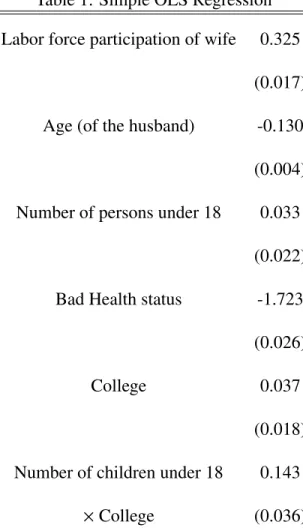
To see how the dependence of the labor force participation on number of children differs across groups of heads of different education level, I estimate a simple, reduced-form model of labor force participation by using CPS (Current Popula- tion Survey)3. The dependent variable is hours worked, and the independent vari- ables are age of the head, monetary assets, family size, bad health status dummy, college educated dummy, and the cross term of family size and college dummy.
As we can see from Table 1, the number of children in the household matters to the amount of hours worked. In addition, the effect of the number of children for college-educated heads is larger than that of high school-educated heads. The estimate indicates that college-educated heads are more likely to work longer when they have children than high-school educated heads, and the magnitude of the effect is larger than the effect of getting one year older.
Why are college-educated heads more sensitive to the number of children? My guess is that children who have college-educated father are likely to go to college, which indicates children in the household with college-educated heads tend to take longer time to be economically independent. So college-educated heads get stronger incentive to work when they have young children than high
3CPS has much larger sample size than PSID, but does not have any information about the asset. I carried out a regression by using PSID and including monetary asset to the model. The coefficient on the cross term was positive and not small, but not significantly different from 0.
school educated heads.
3 Data
I use PSID to estimate a life-cycle model. PSID is a longitudinal study of a representative sample of U.S. individuals and the family units in US, started with 4800 families in 1968.
Since I estimate income process, transition probability of the family size, and change in asset levels, I need panel data that contains detailed information about individuals around retirement age. So I use PSID.
The life-cycle model that I use regards a household as one decision unit. If the decision of single people is dramatically different from that of married people, estimating the same parameter might be problematic. So I eliminated households with single household head.
4 Model
If age and number of children matter, we have to allow for the life cycle path of consumption and saving. Therefore, to see how age of children affects the retire- ment decision, I estimate a life-cycle model that incorporates consumption/saving decision.
Suppose the household lives for t = 25, 26, . . . , 804.
Current Payoff The current utility at age t is given by U(Ct, Ht, Zt) = 1
1 − η [( Ct
Zt
)γ
(L − Ht− φ1{Mt =1} − ψ1{Ht >0})1−γ ]1−η
4The initial age is assumed to be age 25 so as to avoid considering the choice of going to college or getting married. I assume that all of the household heads are married, and can work if they want.
where Ct is consumption, Ht is hours worked, Zt is family size. Mt is a dummy variable of health status, takes 0 if the health status is ”good” or better, 1 if the health status is ”fair” or worse. The time endowment L is 6000, and there is a cost of bad health φ and fixed cost of working ψ.
I discretize the space of hours worked. Let Ht ∈ {0, 500, 1500, 1000, 2000, 2500} be the choice of the hours worked,
The bequest function is of the form b(AT) = θB
(AT+ K)(1−η)γ
1 − η (1)
where T is the terminal period, and K is a parameter that determines the curvature of this function. I assume T = 80, and no household head dies before the age of 80.
Income Process The income at t is given by
Yt =
WtHtNt if t <62
WtHtNt+ P if otherwise
(2)
where Wt is the wage rate, and the multiplicative error term Nt follows i.i.d. log normal distribution and lnNt ∼ N(0, σ2ǫN). I assume that the log wage rate ln Wt depends on the education level, the age, and the health status. The log of wage rate follows
ln Wt = α0+α11{Colleget =1} + α2t + α3t2 (3) + α4t × 1{Colleget =1} + α5t2×1{Colleget =1} + α61{Mt =0},
(4) where College is college-educated dummy that takes 1 if the grades completed is higher than 12. For simplicity, I assume pension P is the deterministic and everyone gets P every period after the age of 625.
5Since only 13of heads have pension and the variance is huge, this simplification involves a serious problem. I will deal with this problem in the future.
The spousal income, YSt, depends only on the head’s age:
ln YtS = ζ0+ ζ1t + ζ2t2. (5)
Social Security After the age of 62, the household heads can draw social se- curity benefit sst. To incorporate social security system precisely in the model, I have to introduce the level of AIME as a continuous state variable. Adding a continuous state variable is costly in a sense that we have to discretize the space and the computation time explodes. To avoid this problem, I assume that the level of the benefit depends only on the education level and the age at which the head started drawing the social security benefit. In addition, I assumed that the Social Security benefit is constant after age 65. The Social Security benefit is determined by
sst = ι0+ ι1College + ι21{Age < 65} + ι31{Age ≥ 65} + ǫt (6) where Age is the age at which the household head started drawing the social security benefit, and takes 65 if the head start drawing after age 65.
Budget Constraint I assume that there is a borrowing constraint and asset cannot be smaller than −10000. In addition, I assume that the household heads cannot leave debt when they die. The budget constraint at age t is given by
At+1 = RAt+ Yt+ YtS + sst−Ct, At+1 ≥ −10000, AT ≥0, (7) where R is gross interest rate, and Atis the asset level at t. I assume ssttakes 0 if the household head has not started drawing the social security benefit yet.
Transition equation of Zt For simplicity, I assume the transition of the num- ber of children is purely stochastic. The family size Zt increases when a child is born, or a child comes back to the household. I assume that Ztchanges according to the following rule;
1. Zt does not decrease if Zt =2, and does not increase if Zt =6.
2. If Zt is greater than 2, then
Zt =
Zt−1−1 with probability PCLt Zt−1 with probability 1 − PCLt
(8)
where PCLtis the probability of a child to become economically indepen- dent. I assume PCLt depends on the age, the education level of the house- hold head. In addition, I assume that PCLt of the older group is different from that of the younger group.
3. If Zt is smaller than 6, then
Zt=
Zt−1+1 with probability PCBIt+ PCBAt Zt−1 with probability 1 − (PCLIt+ PCBAt)
(9)
where PCBIt is the probability of childbirth and PCBAt is the probability of a child to come back. I assume PCBIt and PCBAt depends on the age, the education level of the household head. In addition, I assume that PCBIt
and PCBAt of the older group is different from that of the younger group.
Transition equation of Mt Let Πt be a transition matrix of the Markov pro- cess of health status and
• (1, 1) th element of Πt, π11t, indicates the probability of health status not to change, and to be “good” at period t and t + 1.
• (1, 2) th element of Πt, π12t, indicates the probability of health status to change from “good” to “bad”.
• (2, 1) th element of Πt, π21t, indicates the probability of health status to change from “bad” to “good”.
• (2, 2) th element of Πt, π22t, indicates the probability of health status not to change, and to be “bad” at period t and t + 1.
I assume that the transition probability of health status depends on the age of household head and current health status, and the probability of the transition of
health status follows:
π12t = Φ(κ11+ κ12t) (10)
π21t = Φ(κ21+ κ22t) (11)
where Φ(.) is the c.d.f. of standard normal distribution.
Bellman Equation Let dt be the discrete choice of hours worked and social security draw. Let Vjtbe the value at t when the household choose dt= j, that is,
Vjt(At, Zt, Mt) = max
Ct
U(Ct, Ht, Mt, Zt|dt = j)
+ βEt[Vt+1(At+1, Zt+1, Mt+1)|At, Ct, Zt, Mt, dt = j] s.t At+1= RAt+ Yt+ YSt+ sst−Ct, At+1 ≥0 Vt(At, Zt, Mt, Nt) = max{V1t(At, Zt, Mt), V2t(At, Zt, Mt), V3t(At, Zt, Mt), . . . } I solve the dynamic programming problem by backward induction6
5 Estimation
Estimation Procedure I take a two-step estimation procedure. At first, I estimate the parameters in the wage function (α), spousal income function (ζ) , the transition probability of the family size (PCLt, PCBIt, PCBAt), and the transition probability of health status (Πt) by estimation with reduced-form models.
Using the estimates of the parameters obtained at the first step, I estimate the preference parameters (γ, η, φ, ψ, θ) by using indirect inference. The auxiliary
6 I calculate Vt(At, Zt, Mt, Nt) for each period and each value of At, Zt, Mtand Nt. Then I pick up the quadrature point on the space of Nt so that I can use Gauss-Hermite quadrature to approximate Et−1[Vt(At, Zt, Mt, Nt)]. And finally I use cubic-spline to interpolate Et−1[Vt(At, Zt, Mt, Nt)] so that I can find the optimal consumption by applying the Newton’s Method to the first order condition. I discretized the space of Atin 12 grids, and the degree of Gauss-Hermite quadrature is 6.
model is
Hit= ω1+ ω2t + ω3Ait+ ω4Zit+ ω5Mit+ ω6Collegei+ ut (12)
Ait= ω71{t = 55} + ω81{t = 56} + · · · + ω191{t = 67} (13)
Hit= ω201{t = 55} + ω211{t = 56} + · · · + ω321{t = 67} (14) I use the inverse of variance-covariance matrix7for the weighting matrix W. The objective function is (ωN − ω(θ))′W(ωN − ω(θ)) where ωN is the estimate of ω obtained from the actual data, while ω(θ) is the estimate of ω obtained simulated data.
Identification Previous literatures that use Simulated Method of Moment es- timate β, η, and θBfrom Equation 13.
The cost of bad health, φ, is identified from the sensitivity of Ht to the bad health status. So it should be identified from ω5 in Equation 12. The fixed cost of working, ψ, affects hours worked and the slope of the life-cycle path of hours worked. Thus ψ are likely to be identified through Equation 12 and Equation 138
6 Results of Estimation
6.1 The Results of 1st Step Estimation
Wage Function I assume that the labor force participation choice is approxi- mated by the Probit model, and estimate the wage function (see equation (4)) by
7I obtained variance covariance matrix by boot-strapping.
8To see if the parameters be identified, I estimate the parameters by using simulated data. The estimates was close to the values of the parameters used to generate the data.
using Heckman 2 step procedure9.
I assume that the number of children in the household matters only to the labor force participation, but it doesn’t have any effect on the wage rate. I use this assumption as an exclusion restriction.
Spousal Income I estimate the spousal income function by OLS.
Transition of Health Status I estimated the probit model of the change in health status.
The results indicates that the health status is more likely to be worse as the household heads get older, and they are less likely to recover as they get older.
Transition of Family Size To get the transition probability of family size, PCLt,PCBIt, I impose the following assumptions.
1. the children leave the household no later than the age of 2710. 2. the children can come back if they are younger than the age of 27.
3. I regard those whose labor force participation status changed from “student” or “not working” to “working” as children who left the household.
4. I regard those whose labor force participation status changed from “work- ing” to “not working” as children who came back to the household.
9 I impose this assumption for simplicity. Since the model does not imply that the labor force participation can be represented by the Probit model, this assumption is not internally consistent. So I should use non-parametric Heckman 2 step to deal with the inconsistency.
10I imposed this assumption because the employment status is observable until 1997, though I focus on the children born in 1960s.
Then I calculated PCLt by the following way11: Prob( a child leave the household |t, College)
= Prob( the head have a child of age 18 |t, College)
×Prob(18-year-old man start working |College) + Prob( the head have a child of age 19 |t, College)
×Prob(19-year-old man start working |College) + . . .
I calculated PCBAtin the same way.
Since PSID have information on the year of childbirth, I divide the average number of heads who got children by the number of heads at each age and regard it as PCBIt.
Figure 5 shows how the transition probability of the family size.
6.2 The Results of 2nd Step Estimation
Table 6 gives the estimates of structural parameters that I estimated at the 2nd step12.
11Note that College is the indicator of college-educated head, and do not indicate the education level of the child.
12 The standard error θB seems too large. It may be because the minimization procedure for the estimation converges to a local minimum. I estimated the values of parameters by using simulated data and find that, when the value of the parameter is far from true value, the objective function of estimation is ”flat” in a sense that the value of function does not change when θBchanges a lot.
Figure 5: The Probability of Family Size Change
0 0.05 0.1 0.15 0.2 0.25 0.3
15 20 25 30 35 40 45 50
Age Older Group Younger Group
0 0.05 0.1 0.15 0.2 0.25 0.3
15 20 25 30 35 40 45 50
Age Older Group Younger Group
0 0.05 0.1 0.15 0.2 0.25 0.3
35 40 45 50 55 60 65 70 75 Age
Older Group Younger Group
0 0.05 0.1 0.15 0.2 0.25 0.3
35 40 45 50 55 60 65 70 75 Age
Older Group Younger Group
0 0.05 0.1 0.15 0.2 0.25 0.3
35 40 45 50 55 60 65 70 75 Age
Older Group Younger Group
0 0.05 0.1 0.15 0.2 0.25 0.3
35 40 45 50 55 60 65 70 75 Age
Older Group Younger Group
7 Simulation-Based Analyses and Conclusion
By using the estimated model, I carry out two simulations; one starts from the initial distribution of family size at age 25 of those who were born in 1923-1932, and the transition probability of the family size PCLt,PCBIt, and PCBAt are cal- culated from their history. The other starts from the initial distribution of family size at age 25 of those who were born in 1933-1942, the transition probability of the family size PZt PCLt,PCBIt, and PCBAt are calculated from their history. In order to extract the effect of age and number of children, I assumed both start from the same asset level and face the same income profile over the life-cycle.
Figure 6: Simulation Result: Average of Asset Levels at Each Age
0 20 40 60 80 100 120 140 160 180 200
20 30 40 50 60 70 80
Age
data whole older group younger group
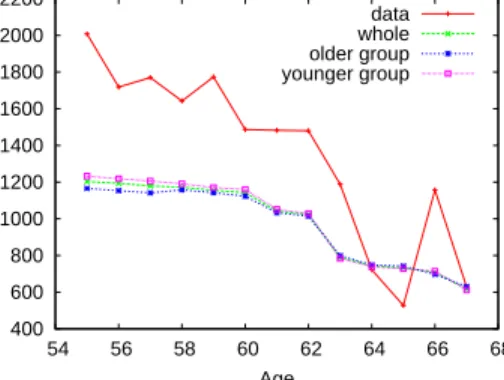
Figure 7: Simulation Result: Average of Hours Worked at Each Age
400 600 800 1000 1200 1400 1600 1800 2000 2200
54 56 58 60 62 64 66 68
Age
data whole older group younger group
Figure 6 shows the average of asset levels at age 55 through 67. It suggests that the the older group of heads accumulate asset more than the younger group of heads do.
So we expect the household heads in the younger group are likely to retire later. I plot the average hours of work on Figure 7. Figure 7 indicates that the household the younger group of heads are likely to retire later than the older group of heads, but the difference is quite small. This result indicates that it is difficult to explain the increase in the labor force participation in the 1990’s by the change in age and number of children.
References
[1] French, E. (2005) “The Effects of Health, Wealth, and Wages on Labor Sup- ply and Retirement Behavior,” Review of Economic Studies,72, No.2, 395- 437
[2] Rust, J. and C. Phelan (1997) “How Social Security and Medicare Affect Retirement Behavior in a World of Incomplete Markets,” Econometrica, 65, No.4, 781-831
[3] Shirle, T. (2008) “Why Have the Labor Force Participation Rates of Older Men Increased since the Mid-1990’s?”, Journal of Labor Economics, 26, No. 4, 549-594.
[4] Sholz J. K. , A. Seshadri , and S. Khitatrakun (2010) “Are Americans Saving Optimally for Retirement? ” Journal of Political Economy, 114, No.4, 607- 643
Table 1: Simple OLS Regression Labor force participation of wife 0.325
(0.017) Age (of the husband) -0.130
(0.004) Number of persons under 18 0.033
(0.022) Bad Health status -1.723
(0.026)
College 0.037
(0.018) Number of children under 18 0.143
×College (0.036)
NOTE-The dependent variable is a dummy variable of labor force participation of household heads. The standard errors are in parentheses. The data is Current Population Survey from 1992 to 2001.
Bad Health and College are dummy variables.
Table 2: Estimation of Wage Function
Constant -0.0059
(0.0415 ) College dummy 0.1944
(0.0880 )
Age -0.0885
(0.0019)
Age2 -0.0009
(0.0000) Age × College dummy -0.0254
(0.0042) Age2×College dummy -0.0002
(0.0000) Health status (=good) 0.2857
(0.0415)
NOTE.- Dependent Variable is ln(Wage Rate)
Table 3: Estimation of Spousal Income Function
Constant -5.1262 (8.3870) Age of husband 0.4897
(0.2804) (Age of husband)2 -0.0042
(0.0023)
NOTE.- The dependent varialbe is ln(labor Income of Wife) .
Table 4: Estimation of Social Security Benefit Function
Constant 4153.477
(204.451 ) Age of starting SS draw 423.606
(86.984 ) The Dummy of Age of starting SS draw ≥ 65 1774.073 (238.6299 )
College dummy 137.050
(80.983 )
NOTE.-The dependent varialbe is social security benefit
Table 5: Estimation of the Prob. of Health Status Change
Change in Health Change in Health from “good” to “bad” from “bad” to “good”
Constant -2.5110 1.2191
(0.014) (0.0215)
Age of head 0.0267 -0.0321
(0.0005) (0.0010)
NOTE.- The dependent variable of the first column is a dummy variable that indicate the change in health status from good to bad, while the second column indicates
the change in health status from bad to good
Table 6: Estimates of Structural Parameters
The weight on consumption γ 0.6071 (1.3982 ) The relative risk aversion coefficient η 0.0298
( 2.4576) The fixed cost of bad health φ 0.4379
(1.4515 ) The fixed cos of working ψ 0.2529
( 0.8010) The weight on the bequest function θB 1.1479
(1.8173 )