The Effect of Bank Recapitalization Policy on Corporate
Investment: Evidence from a Banking Crisis in Japan
∗Hiroyuki Kasahara† University of British Columbia
Yasuyuki Sawada University of Tokyo
Michio Suzuki University of Tokyo
September 1, 2016
Abstract
This article examines the effect of government capital injections into financially trou-bled banks on corporate investment during the Japanese banking crisis of the late 1990s. By helping banks meet the capital requirements imposed by Japanese banking regula-tion, recapitalization enables banks to respond to loan demands, which could help firms increase their investment. To test this mechanism empirically, we combine the balance sheet data of Japanese manufacturing firms with bank balance sheet data and estimate a linear investment model where the investment rate is a function of not only firm pro-ductivity and size but also bank regulatory capital ratios. We find that the coefficient of the interaction between a firm’s total factor productivity measure and a bank’s capital ratio is positive and significant, implying that the bank’s capital ratio affects more pro-ductive firms. Counterfactual policy experiments suggest that capital injections made in March 1998 and 1999 had a negligible impact on the average investment rate, although there was a reallocation effect, shifting investments from low- to high-productivity firms.
Journal of Economic Literature Classification Numbers: E22; G21; G28 Keywords: Capital injection; Bank regulation; Banking crisis
∗Part of this work was done while the first author was a visiting scholar and the third author was
affiliated with the Institute for Monetary and Economic Studies of the Bank of Japan. The authors are grateful for helpful comments received at the Bank of Japan and at numerous conferences and seminars. The authors would like to thank Patrick Bolton, Nobuyuki Kinoshita, Daisuke Miyakawa, Kazuo Ogawa, Alex Popov, Mark M. Spiegel, David Vera, and Philip Vermeulen for their helpful comments. Ai Fujiki, Takafumi Kawakubo, Saori Nishimura, Tomohiro Hara, and Shunsuke Tsuda provided excellent research assistance to create the matched firm–bank data used in this paper. The first author gratefully acknowledges financial support from the Social Sciences Humanities Council of Canada, the second author gratefully acknowledges financial support from JSPS Grant-in-Aid for Scientific Research (S) 26220502, and the third author gratefully acknowledges financial support from Japan Center for Economic Research and JSPS Grant-in-Aid for Young Scientists B No. 22830023. All remaining errors are our own. Views expressed in this paper are those of the authors and do not necessarily reflect the official views of the Bank of Japan.
†Corresponding author. Mailing address: Department of Economics, University of British Columbia,
997 - 1873 East Mall, Vancouver, BC V6T 1Z1, Canada. Tel. 604-822-4814; fax: 604-822-5915; E-mail:
1
Introduction
This paper examines the effect of government capital injections into financially troubled
banks on the level of firm investment during the Japanese banking crisis. During the
banking crisis of 1997, under the risk-based capital requirements imposed on banks, Japan
experienced a sharp decline in bank loans to firms and Japanese corporate investments fell
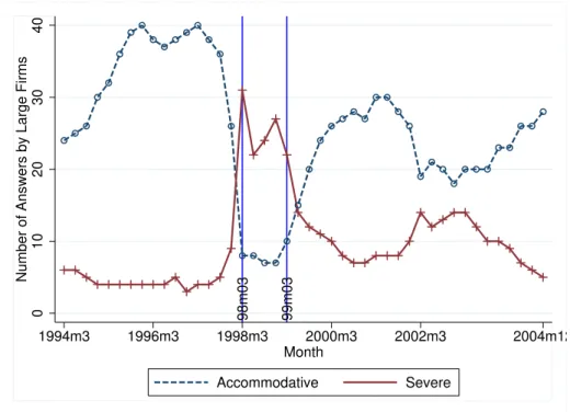
in 1998 and 1999. According to the Short-Term Economic Survey of Enterprises in Japan
(TANKAN) of the Bank of Japan, there was a sharp deterioration of “banks’ willingness
to lend” during the first quarter of 1998 (Figure 1). To cope with the banking crisis, the
Japanese government made capital injections of 1.8 trillion Japanese yen in March 1998 and
7.5 trillion Japanese yen in March 1999 into the top city, trust, and long-term credit banks
and other regional banks in the form of purchases of preferred stock or subordinated debt
or as subordinated loans. These capital injections helped many banks improve their capital
ratios and attain the capital standard required under the 1988 Basel Accord (Basel I) .1
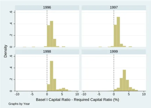
As Figure 2shows, the distribution of the regulatory capital adequacy ratio, which we call
the Basel I capital ratio (BCR), weighted by loan supply across banks substantially shifted
upward from 1997 to 1999.
One of the primary goals of the capital injection plan in Japan was to promote firm
investment by improving bank capital ratios in the hope of increasing bank lending to
firms (Montgomery and Shimizutani (2009)). Did the capital injection promote investments in Japan? If so, how large was the effect? Given that over 10 trillion yen of Japanese
taxpayer money (roughly 2% of Japan’s nominal gross domestic product) was spent on
capital injections into troubled banks, these are important policy questions. However,
while a large body of research investigates whether the credit crunch in Japan constrained
firm investments (Caballero et al. (2008);Hayashi and Prescott (2002);Hori et al. (2006); 1
Hosono (2006);Ito and Sasaki (2002);Motonishi and Yoshikawa (1999);Peek and Rosengren (2000); Woo (2003)), few empirical studies (e.g., Giannetti and Simonov (2013), hereafter GS) quantitatively assess the extent to which government capital injections affected firm
investments by relaxing firms’ financial constraints.
To examine the firm investment effect of the capital injection into banks, we construct a
unique data set, combining Japanese firm-level financial statement data with bank balance
sheet data. Using the matched firm–bank data, we first examine whether capital injections
affect the supply of credit from banks to firms. To examine the effect on corporate
invest-ment, we regress corporate investment on the weighted average of banks’ BCR, as well as
various firm characteristics. We use the BCR because we are interested in a specific
mech-anism: the effect of banks’ BCR on firm investment through financial constraints under
Japanese banking regulations rather than the effect of bank health in general. The use
of the BCR is essential for quantifying the counterfactual policy effect of capital injection
because we can construct the counterfactual value of the BCR without capital injection
from the detailed bank-level information of capital injections in 1998–1999.
Using regression analysis of loan growth on the ratio of the capital injection amount to
bank equity and bank BCR as well as various firm- and bank-level covariates, we find that
the coefficient of the capital injection and that of the bank’s BCR are both positive and
significant. This result indicates that the government capital injections and the higher BCR
help banks to increase their supply of loans to firms. These results are expected because
banks with low BCR have incentive to shift their investment into safer assets like government
bonds under the risk-based capital requirements. Furthermore, the positive coefficient of the
capital injection is consistent with the improvement in banks’ willingness to lend in response
to the capital injections as evidenced in the Bank of Japan’s TANKAN.2 Estimation of a
linear investment model shows that the coefficient of the interaction between the weighted
average of banks’ BCR and the firm-level total factor productivity (TFP) measure is positive
2
and significant. This result suggests that banks’ BCR matters in firms’ investment decisions
when firms are productive and thus have higher demand for investment. Using the estimated
model, we conduct counterfactual experiments to quantify the effect of capital injections
that took place in March 1998 and 1999 in Japan. The counterfactual experiments suggest
that the capital injections had a negligible impact on the average investment rate, although
there is a reallocation effect, with investment shifted from low- to high-productivity firms.
The paper most closely related to ours is that of GS, who also examine the effects of bank
recapitalization policies on the supply of credit and client firm performance, including firm
investment, using matched firm–bank data from the Japanese banking crisis. The authors
find that the size of the capital injection is important for its success: If capital injections are
large enough so that recapitalized banks achieve capital requirements, such banks increase
the supply of credit and firms that borrow from the recapitalized banks increase their
investment. This paper’s contribution beyond that of GS is as follows. First, we examine
whether firms’ loan and investment responses to their banks’ recapitalization depend on
their TFP. This question naturally arises because, theoretically, the higher firm productivity,
the larger firm investment and the demand for external finance tend to be. Therefore,
bank lending attitude, which likely depends on BCR under the banking regulation, may
be more important for high-productivity firms. The finding that high-productivity firms
increase their investments more than low-productivity firms in response to their associated
banks’ recapitalization would suggest that the resource is allocated toward more productive
firms as a result of capital injection.3 Second, we use the BCR as the main variable to
assess the effect of capital injections. Despite the well-known issue of overstating their
net wealth when banks report their capital ratios, examining how the reported BCR is related to firms’ investment decisions is important in this context because it is the reported
BCR that matters under the capital requirements for banks. By focusing on the BCR, our
analysis examines a specific mechanism through which capital injections affects banks’ loan
decisions and firm investment; that is, capital injection helps undercapitalized banks meet
3
the capital ratio requirement specified under Basel I regulations. For a robustness check,
we also report the results based on alternative, conservative measures of BCR that take
into account deferred tax assets as well as defaulted loans. Furthermore, the use of the
BCR facilitates a counterfactual experiment based on the counterfactual value of the BCR
without capital injection.
This paper also contributes to the empirical literature on the effect of financial
con-straints on firm investment (e.g.,Fazzari et al. (1988);Hoshi et al. (1991);Kaplan and Zin-gales (1997)). Empirical papers on the effect of financial constraints use various observed measures of financial constraint, such as cash flow, firm size, and years of establishment,
to examine their effect on investment. It is often difficult, however, to interpret these
em-pirical results because such measures of financial constraint can be viewed as endogenous
variables and correlated with the firm’s efficiency measure, which also explains investment.
For example, a positive estimate of the cash flow coefficient could just reflect its positive
correlation with firm efficiency. This paper examines how the BCR of the bank with which
a firm has a relationship influences the firm’s investment decisions. To the extent that the
BCR measure is viewed as more exogenous than other measures of financial constraint, this
paper’s results shed further light on the impact of financial constraints on investment.
The remainder of this paper is organized as follows. Section 2briefly describes banking
regulations and bank recapitalization policies during the Japanese banking crisis of the
late 1990s. Section3describes our data sources and reports descriptive statistics. Section4
presents our empirical analysis on the effects of capital injection policies on banks’ regulatory
capital ratio, the supply of credit, and corporate investment. Section5concludes the paper.
2
Banking Regulation and Recapitalization Policies in Japan
This section briefly explains banking regulations, particularly the Prompt Corrective Action
scheme and recapitalization policies for banks during Japan’s banking crisis in the late
1990s.4 Recognizing a large amount of non-performing loans accumulated in the financial
4
sector after the collapse of asset prices, as early as 1995, the Ministry of Finance started
discussing a Prompt Corrective Action scheme with which the government could order
undercapitalized banks to take remedial action.5 In December 1996, the Ministry of Finance
published the basic framework of the Prompt Corrective Action that was set to take effect
in April 1998. In preparation, many banks tried to improve their regulatory capital ratio, on
which the regulations were based. Because one way to do so was to decrease risky assets such
as corporate loans, the government was concerned about creating a credit crunch. Therefore,
the government decided to allow some flexibility for banks in the scheme’s implementation.
For example, banks were allowed to choose between market and book values for their stocks
and real estate holdings so that they did not have to report unrealized losses on securities
in their trading account or they could include unrealized capital gains in their real estate
assets in their capital. With such changes in place, the government officially introduced the
Prompt Corrective Action in April 1998.
For banks with international operations, the regulation applies the risk-based capital
adequacy ratio specified in the Basel I capital requirements. The BCR is defined as
BCR= Tier I + Tier II + Tier III−Goodwill Risk weighted asset .
Tier I capital, or core capital, mainly consists of equity capital and capital reserves. Tier II
capital consists of 45% of unrealized capital gains on equity, 45% of the difference between
any revalued land assets and their book value, general loan loss provisions (up to 1.25% of
the risk-weighted asset), nonperpetual subordinated debt, and preferred stocks with more
than five years to maturity. Tier III capital consists of (short-term) subordinated debt with
more than two years to maturity. The sum of Tier II and Tier III capital cannot exceed Tier
I capital. Risk-weighted assets are the weighted sum of bank assets, with weights determined
by the credit risk of each asset class plus a market risk component. For banks with only
domestic operations, domestic capital standards apply, where the risk-based capital ratio is
5
modified as follows:
BCRdomestic=
Tier I + Tier II−Goodwill Risk Weighted Asset .
The definitions of the capital components and risk-weighted assets are the same as above,
except that Tier II capital does not include unrealized capital gains from securities, which
can now be subtracted from risk-weighted assets, general loan loss reserves can be counted
only up to 0.625% of risk-weighted assets, and risk-weighted assets do not include the market
risk component.
Banks with international operations are required to keep their BCR above 8%, while
the minimum capital requirement for domestic banks is 4%. If banks cannot meet these
capital requirements, the Prompt Corrective Action enables the government to order these
banks to restructure or terminate business, depending on their capital ratios.
In November 1997, before the introduction of the Prompt Corrective Action, Sanyo
Securities, Yamaichi Securities, Hokkaido Takushoku Bank, and Tokuyo City Bank failed.6
In response to these failures, the Diet passed the Financial Function Stabilization Act,
which allowed the government to use 30 trillion yen of public funds. Then, in March 1998,
the Japanese government injected 1.8 trillion yen into all of the major (city) banks, as
well as several regional banks. In this capital injection, all the major banks received 100
billion yen through subordinated debt, except for Dai-Ichi Kangyo Bank, which received
99 billion yen through preferred shares. In the fall of 1998, the Financial Supervisory
Agency conducted an intensive examination of the assets of 19 major banks and concluded
that the previous assessment was too optimistic. In October 1998, the Diet passed the
Prompt Recapitalization Act, which doubled the amount of funds to 60 trillion yen. In
October and December of 1998, however, the Long-Term Credit Bank of Japan (LTCB)
and Nippon Credit Bank (NCB) were nationalized. To stabilize the banking sector, the
Japanese government conducted a second round of capital injection into banks, with 7.5
trillion yen in March 1999. Detailed data on the amount of capital injection each bank
6
received are publicly available.7 Therefore, we are able to calculate counterfactual capital
ratios without capital injections by subtracting the injected amounts from the bank capital.
3
Data Source and Variable Definition
To examine the effect of government capital injections into banks on corporate investment,
we combine corporate investment data with bank balance sheet data.8 For corporate balance
sheet information, we use the data set compiled by the Development Bank of Japan (DBJ).
Because the DBJ data set does not contain data for financial institutions, we obtain data on
bank balance sheet information from Nikkei NEEDS Financial Quest (Nikkei NEEDS) and
the “Analysis of Financial Statements of All Banks” by the Japanese Bankers Association
(JBA).
The DBJ data set contains detailed financial statement information for (non-financial)
firms publicly traded in Japanese stock markets. In particular, it provides data on fixed
assets at the component level, such as land, building, and machinery. Furthermore, it
provides data on outstanding loans by financial institutions, which we use to combine with
the Nikkei NEEDS and JBA data.9 Nikkei NEEDS and the JBA provide data on bank
BCRs and non-performing loans, as well as standard bank balance sheet information.10
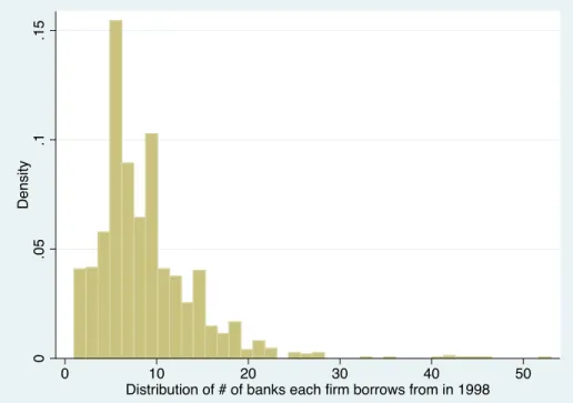
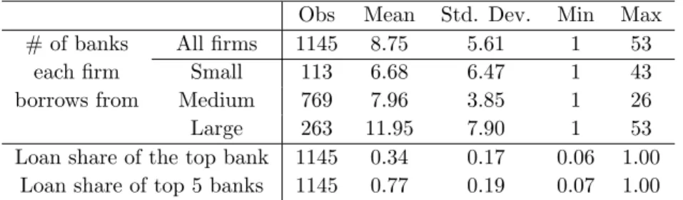
In a given year, each firm borrows from multiple banks. Table 1 and Figure 3 present,
respectively, the statistics and a histogram of the number of banks each firm borrows from in
1998, where we exclude financial institutions other than private banks, such as government
financial institutions and insurance companies, from the observations. The number of banks
each firm borrows from substantially varies across firms, with some borrowing from only
one bank and one firm borrowing from 53 banks. The average number of banks is 8.75 and
7
See, for example, Table 5 ofHoshi and Kashyap (2010). The original data can be found at the website of the Deposit Insurance Corporation of Japan.
8
We followNagahata and Sekine (2005)in combining the two data sets. 9
Fiscal year-end months differ across firms, while all banks end their fiscal year in March in our data set. To reflect the timing of capital injections in March of 1998 and 1999, we match firm balance sheet information in yeart+ 1 with bank balance sheet information in yeartif the closing month of the firms is January or February and match firm observations in yeartwith bank observations in yeartotherwise.
10
the number of banks tends to increase with the number of firm employees. The average
loan share of the top bank, that is, the bank from which firms borrow the most , is 34%,
while the average loan share of the top five banks is 77%, where the loan share of bank k
is defined as the ratio of the loan supply from bank k to total outstanding loans from all
financial institutions.
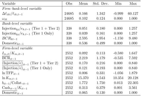
Table 2 reports the summary statistics for the variables in 1997–2000 we use in our
empirical analysis.11 For bank k in year t, we define the variable BCR
kt as the difference
between the bank’s BCR and the required ratio under banking regulations in Japan (8% for
internationally operating banks and 4% for domestically operating banks). To measure the
average BCR of the banks each firm borrows from, for firmiin yeart, we define a variable
BCRit as the weighted average of BCRkt over the banks from which firm i borrows, using
the banks’ outstanding loans in the pre-sample period of 1995–1997 as weights.
Peek and Rosengren (2005) argue that bank health is much better reflected by stock returns than by reported risk-based capital ratios, because Japanese banks hid losses on their
balance sheets using a variety of techniques during the 1990s.12 We use the BCR because we
are interested in a specific mechanism: the effect of the BCR reported in banks’ financial
statements on investments amid financial constraint under Japanese banking regulations
rather than the effect of bank health in general. In this context, the use of the reported
Basel I capital adequacy ratio could be justified to the extent that the banking regulations
directly apply to the BCR reported on banks’ financial statements. Further, the use of
the BCR is essential for quantifying the policy effect of capital injection, because we can
construct the counterfactual value of the BCR without capital injection from the detailed
bank-level capital injection information in 1998–1999 but constructing counterfactual stock
11
Appendix Aexplains in detail how we construct the variables we use in our analysis from the original
data. 12
returns would be difficult.13
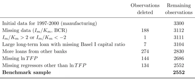
Table3describes our benchmark sample for estimating our firm investment model. We
focus on manufacturing firms. Our main sample period runs from 1997 to 2000, although
we also use data from 1995–1996 to compute the pre-sample period’s loan shares. We
first drop observations missing investment rates or Basel I capital adequacy ratios. We
then drop observations with a machine investment rate (the ratio of machine investment to
machine capital stock) greater than 2 or less than −2. We further drop the observations
of firms that owe more than 20% of total outstanding long-term loans to banks missing
BCR data from Nikkei NEEDS during 1997–2000 . We also drop the observations of firms
that borrowed mainly from the LTCB, NCB, insurance companies, and government financial
institutions, because the LTCB and NCB were nationalized in 1998 and insurance companies
and government financial institutions are not under bank regulations. Finally, we drop
observations missing values for explanatory variables, which leads to a final sample of 2552
observations.
4
Empirical Analysis
4.1 Basel I Capital Adequacy Ratio and Capital Injection in 1998 and
1999
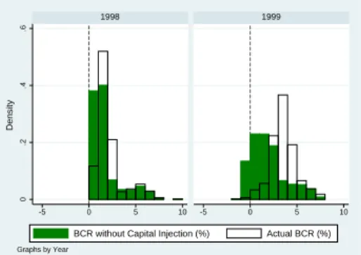
The impact of the capital injections of 1998 and 1999 on the distribution of Basel I capital
adequacy ratios was substantial. In Figure 4, we attempt to construct counterfactual
dis-tributions of BCRktwith no capital injection in 1998 and 1999 and compare them with the
actual distributions weighted by loan supply. The counterfactual value of BCRkt in Figure
4(a) is constructed by subtracting the amount of capital injection from the numerator of
the definition of the Basel I capital adequacy ratio while keeping the denominator, that
is, risk-weighted assets, constant. The counterfactual value of BCRkt in Figure 4(b) is the
13
predicted value of BCR under no capital injection, based on the estimated regression of
BCRkt on BCRkt−1 and Injectionkt/ek,t−1 (Tier 1 + Tier 2) and year dummies, where the
estimated coefficient of Injectionkt/ek,t−1, the ratio of the amount of capital injection into
bank k in year t to its previous year’s equity, is significant at 2.56, with a standard error
of 0.45. The comparison of the constructed counterfactual distributions of BCRktwith the
actual distribution in Figure 4 suggests that, had there been no capital injection in 1998
and 1999, many more banks would have had trouble meeting capital requirements in 1998
and 1999.
If, indeed, the effect of the capital injections of 1998 and 1999 on the Basel I capital
adequacy ratio was substantial, as shown in Figure4, the capital injection must have made
it easier to meet the required capital ratio under Japanese bank regulations, which, in turn,
could have increased the supply of bank loans and promoted firm investment. Next, we
examine the effect of capital injection on the supply of bank loans and firm investment
decisions with regression analysis.
4.2 Bank Loan and Capital Injection
We first examine how capital injection into banks affected the supply of bank loans to
firms using the panel data set from 1995 to 2000. In contrast to the analysis by GS, ours
highlights the role of the Basel I capital adequacy ratio and uses the sample period after
the introduction of Japanese banking regulations on capital ratios. Specifically, we examine
how the size of capital injections to bank k relative to bank’s capital the previous year is
related to the growth rate of loans firm ireceives from bankk by estimating the following
regression for t= 1998, 1999, and 2000:14
∆ℓikt
ℓik,t−1
=β0+β1
Injectionkt
ek,t−1
×ωik
+β2ωik+
Zktb ×ωik
′ βb+
Zitf ×ωik
′ βf
+Dkb +Dfi +Dyeart ×Dclosing monthi +uikt,
(1)
14
where ∆ℓikt/ℓik,t−1 is the growth rate of loans from bank k to firm i in year t. The main
explanatory variables of interest are the amount of capital injection into bank k in year t
relative to its previous year’s equity, denoted Injectionkt/ekt−1, and the difference between
the Basel I capital adequacy ratio and the required ratio under banking regulations at
the end of the previous year, denoted BCRkt−1. In our baseline specification, we include
the average share of bank k’s loans among total loans to firm i in the pre-sample years
(1995–1997), denoted ωik, where we use the pre-sample period’s weights in our baseline
specification to mitigate concerns about the endogenous determination of loan shares. For
a robustness check, we also use the share of bank k’s loans among total loans to firm iin
yeart−1 to defineωik in place of the pre-sample period’s weight. Following GS, we interact
ωik with other explanatory variables.
We include firm and bank dummies, denoted Dfi and Db
k, respectively. Because the
definition of accounting years differs across firms because of different closing months, we
include the interaction term between a year dummy, Dtyear, and a firm-level dummy for
fiscal year closing months, Diclosing month. In our alternative specification, we also consider
the interaction term between the year dummy and the firm dummy, Dyeart ×Dfi, while
dropping the terms Zitf ×ωik and Dyeart ×Dclosing monthi , to check the robustness of the
results in the presence of time-varying firm-level unobservables.
We also include time-varying bank-level variables Zb
kt = (BCRkt−1,Domestickt−1)′ and
firm-level variablesZitf = (lnT F Pit−1,lnKit−1,Cashit−1/Kit−1, bit−1/Collat.it−1)′. The
vari-able Domestickt−1 is a dummy variable that takes the unit value if bank koperates only in
the domestic market in year t−1, lnT F Pit−1 is the log of TFP of firm i in year t−1,15
lnKit−1 is the log of capital stock at the end of year t−1, Cashit−1/Kit−1 is the ratio of
cash holdings to capital stock in year t−1, and bit−1/Collatit−1 is the ratio of total debt
to the collateral value of land and capital stocks.
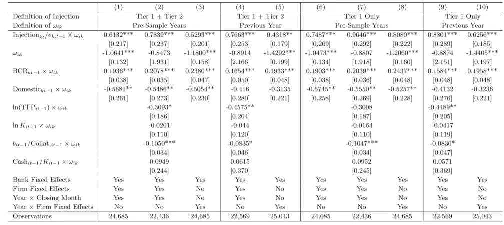
Table 4 presents the estimation results. We use the sum of Tier 1 and Tier 2 capital
injections to compute the variable Injectionkt/ekt−1 in columns (1) to (5), while we only
15
use Tier 1 capital injections in columns (6) to (10). The pre-sample period’s weights are
used for ωik in columns (1) to (3) and (6) to (8), while we check the robustness of our
results using the alternative weights of the share of bankk’s loans to firm i’s total loans in
year t−1 in columns (4) and (5) and (9) and (10). In columns (3), (5), (8), and (10), we
include the interaction of firm fixed effects and the year dummy to control for time-varying
firm-level unobservables.
Across different specifications and alternative measures of capital injection and loan
share weights in Table 4, we find that the coefficient of (Injectionkt/ekt−1)×ωik is
signifi-cantly positive, indicating that banks that received government capital injections increased
their supply of bank loans to firms. Furthermore, the coefficient of BCRkt−1×ωik is positive
and significant and, therefore, banks with a high BCR increased their supply of loans to
firms more than banks with a low BCR did during the financial crisis period of 1998–2000.
Besides a bank’s injection ratio and BCR, the coefficients of lnT F Pit−1 ×ωik and
bit−1/Collatit−1×ωik are negative and significant. Although the latter is expected, the
negative coefficient of firm-level TFP could seem puzzling, because the higher the firm-level
TFP, the higher the demand for investment, which leads to higher demand for external
finance, including bank loans. However, firms with higher TFP are likely to face lower
costs in external financing other than bank loans. Therefore, it could be possible that more
productive firms experience lower loan growth than less productive firms do.16
Although the Prompt Corrective Action regulates the capital ratio of banks, the
re-ported regulatory capital ratio may not fully capture banks’ financial health and could have
overstated their net wealth. We examine the robustness of the results by constructing
al-ternative measures of capital ratios to deal with the known issue of reported capital ratios.
First, following Hoshi and Kashyap (2010) and Nagahata and Sekine (2005), we subtract from bank capital deferred tax assets, which is future tax deductions that banks can claim
for past losses, because deferred tax assets disappear if banks do not have a positive taxable
16
income within five years. Second, we subtract defaulted loans to take into account the
future cost of writing off such loans.
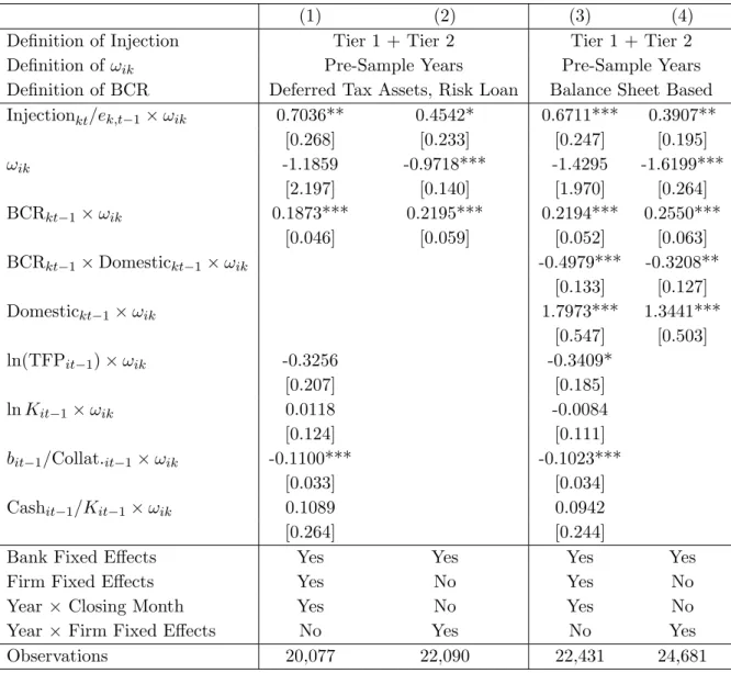
Table5reports the estimation results of the loan growth model with alternative measures
of bank capital ratios. In columns (1) and (2), we modify the regulatory bank capital ratio
by subtracting deferred tax assets and defaulted loans from bank capital. The computation
of this modified capital ratio requires detailed data on bank capital components such as
Tier I and II capital, as well as risk-weighted assets. However, the breakdown data are
not available for some banks, which leads to a smaller number of observations in columns
(1) and (2).17 Thus, in columns (3) and (4), we calculate an alternative bank capital ratio
by using publicly available balance sheet information only so that we can compute the
conservative bank capital ratio adjusted to deferred tax assets and defaulted loans for more
banks. Because it is not appropriate to subtract the minimum capital requirement from the
balance sheet-based capital ratio, we include the variable BCRkt−1×Domestickt−1 ×ωik
to distinguish between international and domestic banks. The estimation results show that
the coefficients of (Injectionkt/ekt−1)×ωik and BCRkt−1×ωik are positive and significant.
4.3 Machine Investment and Capital Injection
We now examine firm machine investment rates. Given the capital requirements imposed by
Japanese banking regulations, financially troubled banks could restrict the supply of credit
to increase their regulatory BCR, which could affect corporate investment when firms are
financially constrained. Our investment model takes into account this potential dependence
of investment on bank capital ratio in addition to standard firm characteristics such as size
and productivity. Specifically, we estimate the following linear investment model:
Im,it
Km,it−1
=α0+α1BCRit−1+α2lnT F Pit−1×BCRit−1+Zit′αf+Dif+D year t ×D
closing month i +ǫit,
(2)
where the dependent variable Im,it
Km,it is the ratio of machine investment in yeartto machine
capital stock in year t−1. The variable BCRit−1 is the weighted average of BCR less the
17
required capital ratio in yeart−1 across the banks firmiborrows from, where the weights
are constructed from the pre-sample loan shares in 1995–1997, computed as BCRit−1 :=
P
kωikBCRkt−1. We also include the interaction of BCRit−1 with lnT F Pit−1 to examine
how the effect of a bank’s BCR depends on firm productivity. The vector Zit contains
ωibankrupt×Dyear99,00, lnT F Pit−1, lnKit−1, Cashit−1/Kit−1,bit−1/Collat.it−1, and Domesticit−1,
where ωbankrupti is the pre-sample share of the LTCB and NCB among firmi’s total loans,
Dyear99,00 is the dummy variable for the period 1999–2000, and Domesticit−1 is the weighted
average of a domestically operating bank’s dummy variable in year t−1, computed as
Domesticit−1 := PkωikDomestickt−1. In the benchmark analysis, we construct data on
lnT F Pit−1 by estimating a firm-level production function with the method proposed by Gandhi et al. (2013). As a robustness check, we also report the results with TFP estimates from the system GMM and the Solow residual in Table7.18
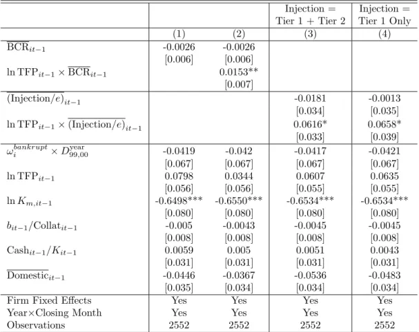
Columns (1) and (2) of Table 6 presents the estimates of equation (2). The coefficient
of BCRit−1 is not significant in column (1), perhaps due to a lack of statistical power, given
that we control for firm fixed effects with a short panel of three years. On the other hand, in
column (2), the significantly positive interaction term between BCRit−1 and the logarithm
of TFP implies that improvements in bank capital ratios could induce larger investments
among firms with higher productivity. Conditioning on capital stock levels, whose estimated
coefficient is significantly negative, we find an increase in productivity to be associated with
higher demand for capital investment but firms are able to invest only if banks are healthy
and willing to supply loans.
We also examine the effect of capital injections on investments by estimating the
follow-ing model:
Im,it
Km,it−1
=α0+α1
Injection e
it−1
+α2lnT F Pit−1×
Injection e
it−1
+Z′
itαf
+Dif+Dtyear×Diclosing month+ǫit,
(3)
where the variable (Injection/e)it := P
kωik(Injectionkt/eit−1) is the weighted average of
18
Appendix Bexplains the estimation method proposed byGandhi et al. (2013)and the system GMM.
the ratio of the sum of Tier 1 and Tier 2 capital injections in year t to bank k’s equity
in year t−1 across banks firmiborrows from, using weights constructed from pre-sample
year loan shares in column (3) of Table 6 and Tier 1 capital injection in place of the sum
of Tier 1 and Tier 2 capital injections in column (4). As shown in columns (3) and (4),
across different specifications and different measures of capital injections, the interaction
of (Injection/e)it with the logarithm of TFP is significantly positive, indicating that the
effect of capital injections into associated banks on firm investment is larger among firms
with higher productivity. This finding suggests that banks that received capital injections
improved their capital ratios and became more willing to lend, which led to an increase in
investments among firms with high productivity growth.
Table7reports the estimation results with alternative bank capital ratios and firm-level
TFP measures. In columns (1) and (2), we examine the effects of the alternative bank
capital ratios adjusted to deferred tax assets and defaulted loans, as in Table 5. Although
the coefficient of ln TFPit−1×BCRit−1 becomes slightly smaller and, likely because of the
smaller sample size, statistically insignificant in column (1), the effect of the interaction term
is larger and statistically significant in column (2). Columns (3) and (4) report results with
alternative firm-level TFP measures constructed by the system GMM and Solow residual,
respectively. These two columns show that the empirical patterns found in Table 6 are
robust, with a positive and significant coefficient of ln TFPit−1×BCRit−1.
Using the estimated models (2) and (3), we quantify the effect on corporate investment
of capital injections that took place in March 1998 and 1999 in Japan. Specifically, we
first compute the counterfactual BCR without capital injections and then calculate the
counterfactual changes in investment rates by taking the difference between the predicted
investment rates based on the actual and counterfactual BCR values.
Table 8reports the mean changes in the investment rates for the whole sample and by
percentiles of ln TFPit−1. In this table, we use the estimates reported in column (2) of
Table6and construct the counterfactual BCR by simply subtracting the injection amounts
from a bank’s Tier I and Tier II capital while keeping risk-weighted assets constant. The
have been 0.2% lower in 1998 and 1.1% lower in 1999 without the capital injections in those
years. For the rest of the firms, however, the investment rates would have been higher. Table 8 also reports the results for alternative measures of bank capital ratios, where we
subtract deferred tax assets and defaulted loans from the regulatory bank capital. With
the alternative measures of the bank capital ratios, the effects of capital injections tend to
be larger. In particular, when we use the bank capital ratio computed based on publicly
available balance sheet information and adjusted to deferred tax assets and defaulted loans,
the investment rates would have been lower for firms with TFP above the 25th percentile
in both 1998 and 1999 and, for firms with TFP above the 90th percentile, the investment
rates would have dropped by 2.5% in 1999.
Table 9 reports the results of the same counterfactual experiments, except that we
now construct the counterfactual BCR without capital injections based on the estimated
regression of the BCR on the lagged capital ratio, the ratio of the injection amount to
equity and year dummies. Table 10 reports the results of the counterfactual experiments
from investment model (3) based on the estimates reported in column (3) of Table (6). The
quantitative effects are similar to those reported in Table8.
5
Conclusion
In this study, we examine the effect of government capital injections into financially troubled
banks on the level of corporate investment during the Japanese banking crisis of the late
1990s. By combining the balance sheet data of Japanese manufacturing firms with banks’
balance sheet data, we first estimate the effects of capital injections and bank regulatory
capital ratios on the growth of loans to firms and confirm that the effects are positive and
significant. Recapitalization policies can promote the investment of client firms if capital
injections help banks respond to loan demands. To test this mechanism empirically, we
model corporate investment as a function of not only standard firm characteristics, such
as size and productivity, but also banks’ regulatory capital ratio. By estimating a linear
capital ratios is positive and significant, suggesting that a bank’s capital ratio matters for
more productive firms. Furthermore, we conduct counterfactual experiments to quantify
the effect of capital injections that took place in March 1998 and 1999 in Japan. The
counterfactual experiments suggest that the capital injections had a negligible impact on
the average investment rate, although there is a reallocation effect, with investment shifting
from low- to high-productivity firms.
Our analysis differs in two important ways from that of GS, who also examine the
effects of bank recapitalization policies on the supply of credit and client firms’ performance,
including firm investment, using data from the Japanese banking crisis. First, we uncover
empirical patterns of how capital injections affect corporate investment by interacting banks’
regulatory capital ratio and capital injection amounts with firms’ TFP. Our estimation
results show that the coefficients of these interaction terms are positive and significant in
the investment regressions. Second, we focus on the specific mechanism of capital injections
helping undercapitalized banks meet the capital requirements imposed by Japanese banking
regulations. To do so, we use banks’ regulatory capital ratio as the main variable to assess
the effect of capital injections. Use of the regulatory capital ratio also enables us to conduct
counterfactual experiments based on the counterfactual values of the regulatory capital ratio
without capital injections.
It is worth noting that the objective of this paper is limited and does not aim to examine
the effect of capital injection in general. This is an important limitation, because capital
injections are likely to have had important impacts on the Japanese economy through other
mechanisms, such as by promoting the write-off of non-performing loans and stabilizing the
financial system.
Appendix A: Development Bank of Japan Data
The data set compiled by the Development Bank of Japan (DBJ) contains detailed corporate
balance sheet/ income statement data for firms listed on the stock markets in Japan. In
(CGPI) for all goods. If firms change their closing dates, the data after the change may
refer to fewer than 12 months. When this occurs, we multiply the dataxit by 12/m, where
mrepresents the number of months to which the data refer. The rest of this section explains
how we construct variables from the original data.
A.1 Variable Construction
Machine Capital Stock
In the benchmark analysis, we use data on machinery and transportation equipment
as machine capital. We construct the real machine capital stock in the DBJ data by the
perpetual inventory method, followingHayashi and Inoue (1991). First, we construct a series of nominal investments in machinery and transportation equipment. Let (pI)itdenote firm
i’s nominal investment in periodt. LetKbook
it denote the book value of the stock of machine
capital at theend of period t. Let δKbook
it denote a depreciated value of machinery. Then,
we compute (pI)it by the following formula: (pI)it=Kitbook−Kitbook−1 +δKitbook−1.
Second, we deflate the nominal investment data by the CGPI for machinery and
trans-portation equipment. Denote the real investment by Iit. Third, we construct data on real
capital stock by the perpetual inventory method. Let Kit denote firmi’s real capital stock
in period t. Then we compute {Kit}t by Kit+ = (1−δ)Kit+Iit, where the depreciation
rate, δ, is taken from Hayashi and Inoue (1991). The initial base year is 1969. For firms entering the sample after 1969, we set the base year to their first year in the sample. We
assume that the book value is equal to the market value for the base year and deflate the
book value by the corresponding CGPI. If the stock value becomes negative in the perpetual
inventory method, we reset the stock value to the book value for the year. We multiply real
capital stock by the corresponding CGPI series to obtain data on machine capital stock in
current yen.
Land Stock
evaluate inventory, we construct nominal investment as follows:
(pI)it =
Kbook
it −Kitbook−1 if Kitbook ≥Kitbook−1
(Kbook
it −Kitbook−1)(plandt /plands ) if Kitbook< Kitbook−1,
wherepland
s is the price of land at which land was last bought (Hoshi and Kashyap (1990); Hayashi and Inoue (1991)).
With the nominal investment series and the depreciation rate, which is set to zero,
we construct data on the nominal stock of land through the perpetual inventory method,
(pK)it = (pt/pt−1)(pK)it−1 + (pI)it, where (pK)it represents the value of firm i’s land
stock in current yen in period t, (pI)it is the value of land investment in current yen, and
pt is the price of land in period t. For the base year, we use a book-to-market ratio to
convert the book value of land stocks into their market value. For the book-to-market
ratio, following Hayashi and Inoue (1991), we use an estimate of the market value of land owned by non-financial corporations from the National Income Accounts and the book value
from Corporate Statistics Annual.
Net Debt
For debt, we use the sum of short- and long-term borrowing and corporate bonds. Net
debt is then computed by subtracting the amount of deposits from the debt.
Output
The nominal output for periodtis total sales plus changes in the inventories of finished
goods.
Appendix B: Estimation of Production Function
B.1 Gandhi, Navarro, and Rivers, 2013 (GNR)
This section briefly explains the estimation procedure proposed by GNR . Consider
Yit = exp(ǫit)Qit
withωit =h(ωit−1) +ηit, whereYitis realized output,Litis labor input,Kitis capital stock,
Mit is intermediate input, ǫit is an unexpected idiosyncratic shock that is unknown when
the input choiceMitis made in period t, andηit is an innovation toωit that is unknown in
period t−1 but known when the input choice Mit is made in periodt. The shocksǫit and
ηit are independent and identically distributed, with mean zero and standard deviationsσǫ
andση, respectively. In what follows, we denote the logarithmic values of (Yit, Lit, Kit, Mit)
by (yit, ℓit, kit, mit).
We assume that Mit is a flexible input. As GNR discuss, the identification problem
arises becausemit is a deterministic function of (ωit, kit, ℓit) and there is no cross-sectional
variation that will allow us to identify the coefficient ofmit once (ωit, kit, ℓit) is conditioned
on. To deal with the identification problem, we exploit the first-order condition with respect
toMit. The first-order condition is written as follows:
lnPM tMit Yit
= lnGt(Lit, Kit, Mit)E[eǫit]
−ǫit, (4)
where Gt(Lit, Kit, Mit) = FM,tFt(L(Litit,K,Kitit,M,Mitit)M) it. From Gt(Lit, Kit, Mit) = FM,tFt(L(Litit,K,Kitit,M,Mitit)M) it,
it follows that
Ft(Lit, Kit, Mit)e−Ct(Lit,Kit) =e R
Gt(Lit,Kit,Mit)dMitMit
⇔ Ft(Lit, Kit, Mit) =e R
Gt(Lit,Kit,Mit)dMitMit+Ct(Lit,Kit)
.
Then, we have
ωit=yit−
Z
Gt(Lit, Kit, Mit)
dMit
Mit
− Ct(Lit, Kit)−ǫit.
Following GNR, we estimate (4) by nonlinear least squares. In the estimation, we
approximate G(Lit, Kit, Mit) by a polynomial of order two, denoted G2; that is,
G2(Lit, Kit, Mit) =
X
rl+rk+rm≤2
γrl,rk,rml
rl
itk rk
itm rm
it withrl, rk, rm ≥0. (5)
Using estimates of γrl,rk,rm, we obtain the estimate of the residual, denoted ˆǫit. Note that,
ifGis a polynomial of orderr, the integral of Ghas the following closed-form solution:
Gr(Lit, Kit, Mit)≡
Z
Gr(Lit, Kit, Mit)
dMit
Mit
= X
rl+rk+rm≤r
γrl,rk,rm
rm+ 1
lrl
itk rk
itm rm+1
As GNR, we approximateC(Lit, Kit) by a polynomial of order two; that is,
C2(Lit, Kit) =αℓℓit+αkkit+αℓℓℓ2it+αkkk2it+αℓklitkit
Letα= (αℓ, αk, αℓℓ, αkk, αℓk). Define ωit(α) by
ωit(α) =
yit−
X
rl+rk+rm≤2
ˆ γrl,rk,rm
rm+ 1
lrl
itk rk
itm rm+1
it −ǫˆit
−(αℓℓit+αkkit+αℓℓℓ2it+αkkkit2 +αℓklitkit).
Usingωit(α), we define ˆηit(α) by19
ˆ
ηit(α) =ωit(α)−ρ0t−ρ1ωit−1(α).
To estimate α, we use the following moment conditions:
E[zitηit] =0,
wherezit= (ℓit, kit, ℓit2, kit2, ℓitkit).
B.2 System GMM `a la Blundell and Bond (1998, 2000)
We consider the following production function:
yit = α0+αℓℓit+αkkit+αmmit+µi+ηt+ωit+ǫit (6)
ωit = ρωi,t−1+ηit (7)
whereyitis the logarithm of the total gross output,ℓit is the logarithm of labor input,kitis
the logarithm of capital input, andmitis the logarithm of intermediate input. The variable
ωit represents the persistent component of TFP and follows the AR(1) process, whereηit is
independent ofωi,t−1. The variable ǫit is a measurement error.
One of the main econometric issues in estimating the production function (6)-(7) is the
simultaneity of a productivity shock ωit and input decisions. All the input variables, ℓit,
kit, and mit, are likely to be correlated with productivity shock ωit and the ordinary least
squares estimate will be biased.
19
To estimate the production function consistently, we first take a “quasi-difference,”
yit−ρyi,t−1, to eliminateωit and ωi,t−1 as
yit = ρyi,t−1+αℓℓit−ραℓℓi,t−1+αkkit−ραkki,t−1+αmmit−ραmmi,t−1+µi+ηit
= π1yi,t−1+π2ℓit+π3ℓi,t−1+π4kit+π5ki,t−1+π6mit+π7mi,t−1+µi+ηit.
Then, we apply the system GMM estimator of Blundell and Bond (1998) to estimate the parameter vector π = (π1, π2, π3, π4, π5, π6, π7) without imposing cross-parameter
con-straints. We also include the year dummies. Here, kit is a predetermined variable so that
E[∆ωitki,t−s] = 0 holds for s= 1,2, ..., while ℓit and mit are endogenous variables, where
E[∆ωitℓi,t−s] = 0 and E[∆ωitmi,t−s] = 0 hold for s= 2,3, .... We also use additional
mo-ment conditions implied by initial conditions under stationarity. After estimatingπ by the
GMM estimation procedure, we impose cross-parameter restrictions, such as π5 = −ραk,
Figures and Tables
Figure 1: Bank Attitudes toward Lending (TANKAN, Bank of Japan)
98m03 99m03
0
10
20
30
40
Number of Answers by Large Firms
1994m3 1996m3 1998m3 2000m3 2002m3 2004m12
Month
Figure 2: Distribution of Basel I Capital Adequacy Ratios, 1996-1999
0
.2
.4
.6
0
.2
.4
.6
-10 -5 0 5 10 -10 -5 0 5 10
1996 1997
1998 1999
Density
Basel I Capital Ratio - Required Capital Ratio (%)
Graphs by Year
Figure 3: Distribution of the Number of Banks Each Firm Borrows from in 1998
0
.0
5
.1
.1
5
D
e
n
si
ty
0 10 20 30 40 50
Figure 4: Basel I Capital Adequacy Ratios (BCRs) without Capital Injections, 1998 and
1999
0
.2
.4
.6
-5 0 5 10 -5 0 5 10
1998 1999
BCR without Capital Injection (%) Actual BCR (%)
Density
Graphs by Year
(a) Counterfactual BCRs with No Adjustment in Risk-Weighted Assets
0
.2
.4
.6
-5 0 5 10 -5 0 5 10
1998 1999
BCR without Capital Injection (%) Actual BCR (%)
Density
Graphs by Year
(b) Counterfactual BCR Based on Regression Estimates
Table 1: Number of Banks Each Firm Borrows from and Top Bank Loan Shares in 1998
Obs Mean Std. Dev. Min Max # of banks All firms 1145 8.75 5.61 1 53
each firm Small 113 6.68 6.47 1 43 borrows from Medium 769 7.96 3.85 1 26 Large 263 11.95 7.90 1 53 Loan share of the top bank 1145 0.34 0.17 0.06 1.00
Loan share of top 5 banks 1145 0.77 0.19 0.07 1.00
Table 2: Summary Statistics (t= 1998,1999,2000)
Variable Obs Mean Std. Dev. Min Max
Firm–bank-level variable
∆ℓikt/ℓik,t−1 24685 0.166 1.342 -0.999 60.127
ωik 24685 0.102 0.124 0.000 1.000
Bank-level variable
Injectionkt/ek,t−1(Tier 1 + Tier 2) 338 0.051 0.180 0.000 1.257 Injectionkt/ek,t−1(Tier 1 Only) 338 0.039 0.161 0.000 1.257
BCRkt−1 338 2.595 1.954 -1.150 9.480
Domestickt−1 338 0.536 0.499 0.000 1.000 Firm-level variable
Im,it/Km,it−1 2552 0.092 0.113 -0.580 1.647
BCRit−1 2552 2.219 1.179 -0.535 7.592
(Injection/e)it−1(Tier 1 + Tier 2) 2552 0.170 0.216 0.000 0.840 (Injection/e)it−1(Tier 1 Only) 2552 0.121 0.193 0.000 0.840 ln TFPit−1 2552 0.006 0.331 -1.056 1.879 lnKm,t−1 2552 15.370 1.543 10.354 20.128 bit−1/Collat.it−1 2552 1.772 1.750 0.013 22.305 Cashit−1/Kit−1 2552 0.313 0.379 0.001 3.561 Domesticit−1 2552 0.065 0.130 0.000 1.000
Notes: The summary statistics forFirm–bank-level variable andBank-level variableare computed from the
firm–bank observations and bank observations used in estimating column (3) of Table 4. The summary statistics for the other firm-level variables are computed from the firm-level observations used in estimating Table 6that satisfy the sample selection criteria reported in Table3. The variable ∆ℓikt/ℓik,t−1 denotes the growth of loans of bankkto firmibetween yearst−1 andt;ωikis the average share of bankk’s loans among total loans to firmiin the pre-sample years (1995–1997); Injectionkt/ek,t−1 (Tier 1 + Tier 2) is the amount of capital injection into bankk’ Tier 1 and Tier 2 capital in yeartrelative to its previous year’s equity; Injectionkt/ek,t−1 (Tier 1 only) is the ratio of the capital injection amount into Tier 1 capital to the bank’s previous year’s equity; BCRkt−1 is the difference between the bank’s BCR and the required ratio under Japanese banking regulations; Domestickt−1 is a dummy variable that takes the value of one if bankkoperates only in the domestic market in yeart−1;Im,it/Km,it−1 is the ratio of firmi’s investment to its previous year’s assets; BCRit−1 is the weighted average of BCRkt over the banks from which firm i borrows; (Injection/e)it−1 (Tier 1 + Tier 2) is the ratio of the weighted average of Tier 1 and Tier 2 injections to equity; (Injection/e)it−1(Tier 1 only) is the ratio of the weighted average of Tier 1 injection to equity; ln TFPit−1is the logarithm of firmi’s TFP in yeart−1;bit−1/Collat.it−1 is the ratio of total debt to the collateral value of land and capital stocks of firmiin yeart−1; Cashit−1/Kit−1 is the ratio of firm
Table 3: Benchmark Sample Selection for Firm Investments Model
Observations Remaining deleted observations
Initial data for 1997-2000 (manufacturing) 3300
Missing data (Im/Km, BCR) 188 3112
Im/Km >2 or Im/Km <−2 1 3111
Large long-term loan with missing Basel I capital ratio 7 3104
More loans from other banks 274 2830
Missing lnT F P 144 2686
Missing regressors other than lnT F P 134 2552
Benchmark sample 2552
Table 4: Effect of Government Capital Injections on Bank Loans (Dependent Variable ∆ℓikt
ℓik,t−1)
(1) (2) (3) (4) (5) (6) (7) (8) (9) (10)
Definition of Injection Tier 1 + Tier 2 Tier 1 + Tier 2 Tier 1 Only Tier 1 Only
Definition ofωik Pre-Sample Years Previous Year Pre-Sample Years Previous Year
Injectionkt/ek,t−1×ωik 0.6132*** 0.7839*** 0.5293*** 0.7663*** 0.4318** 0.7487*** 0.9646*** 0.8080*** 0.8801*** 0.6256***
[0.217] [0.237] [0.201] [0.253] [0.179] [0.269] [0.292] [0.222] [0.289] [0.185]
ωik -1.0641*** -0.8473 -1.1800*** -0.8914 -1.4292*** -1.0473*** -0.8807 -1.2060*** -0.8874 -1.4405***
[0.132] [1.931] [0.158] [2.166] [0.199] [0.134] [1.918] [0.160] [2.151] [0.197]
BCRkt−1×ωik 0.1936*** 0.2078*** 0.2380*** 0.1654*** 0.1933*** 0.1903*** 0.2039*** 0.2437*** 0.1584*** 0.1958***
[0.038] [0.035] [0.047] [0.050] [0.048] [0.038] [0.036] [0.048] [0.048] [0.048]
Domestickt−1×ωik -0.5681** -0.5486** -0.5054** -0.416 -0.3135 -0.5745** -0.5550** -0.5257** -0.4132 -0.3236
[0.261] [0.273] [0.230] [0.280] [0.221] [0.258] [0.269] [0.228] [0.276] [0.221]
ln(TFPit−1)×ωik -0.3093* -0.4575** -0.3008 -0.4489**
[0.186] [0.204] [0.187] [0.205]
lnKit−1×ωik -0.0201 -0.044 -0.0164 -0.0417
[0.110] [0.120] [0.110] [0.119]
bit−1/Collat.it−1×ωik -0.1050*** -0.0835* -0.1047*** -0.0830*
[0.034] [0.046] [0.034] [0.047]
Cashit−1/Kit−1×ωik 0.0949 0.0615 0.0952 0.0571
[0.244] [0.370] [0.245] [0.369]
Bank Fixed Effects Yes Yes Yes Yes Yes Yes Yes Yes Yes Yes
Firm Fixed Effects Yes Yes No Yes No Yes Yes No Yes No
Year×Closing Month Yes Yes No Yes No Yes Yes No Yes No
Year×Firm Fixed Effects No No Yes No Yes No No Yes No Yes
Observations 24,685 22,436 24,685 22,569 25,043 24,685 22,436 24,685 22,569 25,043
Notes: The matched firm–bank observations fort= 1998, 19999, and 2000 are used for estimation, where the numbers of observations are unbalanced across different specifications because of missing values for some regressors. The dependent variable is the growth rate of loans from bankkto firm i. The variableωik is the average share of bankk’s loans among firmi’s total loans in the pre-sample years from 1995 to 1997 in columns (1) to (3)
and (6) to (8), while we use the share of bankk’s loans to firmi’s total loans in yeart−1 as the weightsωikin columns (4) and (5) and (9) and (10).
The variable Injectionkt/ek,t−1is the ratio of the sum of Tier 1 and Tier 2 capital injections in yeartto bankk’s equity in yeart−1 in columns (1) to (5), while we use Tier 1 capital injections in place of the sum of Tier 1 and Tier 2 capital injections in columns (6) to (10). The variable BCRk,t−1 is defined as the BCR less the required capital ratio (8% for internationally operated banks and 4% for domestic banks) in yeart−1; Domestickt−1 is a dummy variable that takes the unit value if bankkis a domestically operating bank in yeart−1; lnT F P is the logarithm of firmi’s TFP in yeart−1; lnKit−1is the logarithm of capital stock for firmiin yeart−1;bit−1/Collat.it−1 is the ratio of total debt to the collateral values of land
Table 5: Effect of Government Capital Injections on Bank Loans (Dependent Variable
∆ℓikt
ℓik,t−1)
(1) (2) (3) (4)
Definition of Injection Tier 1 + Tier 2 Tier 1 + Tier 2
Definition of ωik Pre-Sample Years Pre-Sample Years
Definition of BCR Deferred Tax Assets, Risk Loan Balance Sheet Based Injectionkt/ek,t−1×ωik 0.7036** 0.4542* 0.6711*** 0.3907**
[0.268] [0.233] [0.247] [0.195]
ωik -1.1859 -0.9718*** -1.4295 -1.6199***
[2.197] [0.140] [1.970] [0.264]
BCRkt−1×ωik 0.1873*** 0.2195*** 0.2194*** 0.2550***
[0.046] [0.059] [0.052] [0.063]
BCRkt−1×Domestickt−1×ωik -0.4979*** -0.3208**
[0.133] [0.127]
Domestickt−1×ωik 1.7973*** 1.3441***
[0.547] [0.503]
ln(TFPit−1)×ωik -0.3256 -0.3409*
[0.207] [0.185]
lnKit−1×ωik 0.0118 -0.0084
[0.124] [0.111]
bit−1/Collat.it−1×ωik -0.1100*** -0.1023***
[0.033] [0.034]
Cashit−1/Kit−1×ωik 0.1089 0.0942
[0.264] [0.244]
Bank Fixed Effects Yes Yes Yes Yes
Firm Fixed Effects Yes No Yes No
Year×Closing Month Yes No Yes No
Year×Firm Fixed Effects No Yes No Yes
Observations 20,077 22,090 22,431 24,681
Table 6: Firm Machine Investment Rates, Basel I Capital Adequacy Ratios, and Capital Injections (Dependent Variable Im,it
Km,it−1)
Injection = Injection = Tier 1 + Tier 2 Tier 1 Only
(1) (2) (3) (4)
BCRit−1 -0.0026 -0.0026
[0.006] [0.006] ln TFPit−1×BCRit−1 0.0153**
[0.007]
(Injection/e)it−1 -0.0181 -0.0013
[0.034] [0.035] ln TFPit−1×(Injection/e)it−1 0.0616* 0.0658*
[0.033] [0.039]
ωibankrupt×D
year
99,00 -0.0419 -0.042 -0.0417 -0.0421
[0.067] [0.067] [0.067] [0.067]
ln TFPit−1 0.0798 0.0344 0.0607 0.0635
[0.056] [0.056] [0.055] [0.055] lnKm,it−1 -0.6498*** -0.6550*** -0.6534*** -0.6534***
[0.080] [0.080] [0.080] [0.080]
bit−1/Collatit−1 -0.005 -0.0043 -0.0045 -0.0045 [0.008] [0.008] [0.008] [0.008] Cashit−1/Kit−1 0.0059 0.005 0.0051 0.0043 [0.031] [0.031] [0.031] [0.031] Domesticit−1 -0.0446 -0.0367 -0.0536 -0.0483 [0.035] [0.034] [0.034] [0.034]
Firm Fixed Effects Yes Yes Yes Yes
Year×Closing Month Yes Yes Yes Yes
Observations 2552 2552 2552 2552
Notes: The matched firm–bank observations for 1998–2000 are used for estimation, where the numbers of observations are unbalanced across different specifications because of missing values for some regressors. The dependent variable is the ratio of machine investment in year tto the beginning-of-period machine capital stock in yeart. The variable BCRit−1 is the weighted average of the BCR less the required capital ratio in yeart−1 across the banks firmiborrows from, where the weight is constructed by the loan share
in 1995–1997. The variable (Injection/e)itis the weighted average of the ratio of the sum of Tier 1 and Tier 2 capital injections in yeartto bankk’s equity in yeart−1 across the banks firm iborrows from, using
weights constructed from pre-sample year loan shares in column (3), while we use Tier 1 capital injections in place of the sum of Tier 1 and Tier 2 capital injections in columns (4). The variablezit−1is the logarithm of firm i’s TFP in yeart−1; lnKm,it is the logarithm of machine capital stock for firmiin year t−1; bit−1/Collat.it−1is the ratio of debt to the collateral value of land and capital stocks for firmiin yeart−1; Cashit−1/Kit−1 is the ratio of cash holdings to capital stocks for firmiin yeart−1; Domesticit−1 is the weighted average of a domestically operating bank’s dummy variable in yeart−1 using the loan share of
Table 7: Firm Machine Investment Rates, Basel I Capital Adequacy Ratios, and Capital
Injections (Dependent Variable Im,it
Km,it−1)
(1) (2) (3) (4)
Adjusted BCR 1 Adjusted BCR 2 System GMM Solow Residual
BCRit−1 -0.0042 0.0002 -0.0017 -0.0022
[0.008] [0.010] [0.006] [0.006] ln TFPit−1×BCRit−1 0.011 0.0177* 0.0144** 0.0144**
[0.007] [0.011] [0.006] [0.006]
BCR×Domesticit−1 0.0145
[0.021] ln TFPit−1×BCR×Domesticit−1 0.0153 [0.021]
ωibankrupt×D
year
99,00 -0.0377 -0.0456 -0.0458 -0.0365
[0.070] [0.069] [0.068] [0.067]
ln TFPit−1 0.0879 -0.0051 -0.0098 -0.0108
[0.057] [0.059] [0.065] [0.059] lnKm,it−1 -0.5962*** -0.6534*** -0.6611*** -0.6540***
[0.079] [0.081] [0.080] [0.080]
bit−1/Collatit−1 -0.0026 -0.0049 -0.0045 -0.0043 [0.009] [0.008] [0.008] [0.008]
Cashit−1/Kit−1 -0.0127 0.0024 0.0102 0.0094
[0.031] [0.031] [0.031] [0.032]
Domesticit−1 -0.0645 -0.0921 -0.0359 -0.0402
[0.052] [0.093] [0.033] [0.033]
Firm Fixed Effects Yes Yes Yes Yes
Year×Closing Month Yes Yes Yes Yes
Observations 2,418 2,543 2,552 2,552
Table 8: Effects of Capital Injections on Average Investment Rates
(1) (2) (3) (4) (5) (6) (7)
ln TFPit−1 All ≤10% (10% 25%] (25% 50%] (50% 75%] (75% 90%] >90% BCRit−1
No 1998 Injection 0.0017 0.0043 0.0035 0.0025 0.0013 0.0001 -0.0021 No 1999 Injection 0.0114 0.0261 0.0201 0.0139 0.0079 0.0003 -0.0113 Adjusted BCR 1
No 1998 Injection 0.0002 0.0008 0.0005 0.0004 0.0002 -0.0002 -0.0011 No 1999 Injection 0.0041 0.0139 0.0096 0.0059 0.0019 -0.0029 -0.0106 Adjusted BCR 2
No 1998 Injection -0.0009 0.0005 0.0001 -0.0004 -0.0010 -0.0017 -0.0028 No 1999 Injection -0.0068 0.0052 0.0001 -0.0043 -0.0100 -0.0163 -0.0245
Notes: Columns (1) to (7) report mean changes in the investment rates by percentile of ln TFPit−1. We construct the counterfactual BCR without capital injections by simply subtracting the amount of capital injections from banks’ Tier I and Tier II capital. The sample for 1998–2000 is used to compute the percentiles of ln TFPit−1. The rows designated No 1998 Injection report the counterfactual mean changes in the investment rates if there was no capital injection in March 1998, while the rows designated No 1999 Injection report the counterfactual mean changes in the investment rates without the March 1999 capital injection.
Table 9: Effects of Capital Injections on Average Investment Rates (Regression-Based)
(1) (2) (3) (4) (5) (6) (7)
ln TFPit−1 All ≤10% (10% 25%] (25% 50%] (50% 75%] (75% 90%] >90% No 1998 Injection 0.0010 0.0027 0.0023 0.0015 0.0008 0.0001 -0.0013 No 1999 Injection 0.0066 0.0151 0.0118 0.0079 0.0045 0.0001 -0.0063 Adjusted BCR 1
No 1998 Injection 0.0004 0.0018 0.0014 0.0008 0.0002 -0.0004 -0.0016 No 1999 Injection 0.0032 0.0107 0.0074 0.0045 0.0014 -0.0023 -0.0078 Adjusted BCR 2
No 1998 Injection -0.0016 0.0010 0.0001 -0.0008 -0.0019 -0.0032 -0.0054 No 1999 Injection -0.0074 0.0055 0.0000 -0.0047 -0.0109 -0.0176 -0.0263
Notes: Columns (1) to (7) report mean changes in the investment rates by the percentile of ln TFPit−1. We construct the counterfactual BCR without capital injections based on the esti-mated regression of the BCR on the lagged capital ratio, the ratio of the injection amount to equity, year dummies, and bank fixed effects. The sample for 1998–2000 is used to compute the percentiles of ln TFPit−1. The rows designated No 1998 Injection report the counterfactual mean changes in
Table 10: Effects of Capital Injections on Average Investment Rates (Column (3), Table6)
(1) (2) (3) (4) (5) (6) (7)
ln TFPit−1 All ≤10% (10% 25%] (25% 50%] (50% 75%] (75% 90%] >90% Based on Col.(3), Table6
No 1998 Injection 0.0001 0.0029 0.0019 0.0009 -0.0002 -0.0015 -0.0037 No 1999 Injection 0.0024 0.0163 0.0105 0.0049 -0.0011 -0.0082 -0.0185
References
Blundell, R. and S. Bond (1998). Initial conditions and moment restrictions in dynamic panel data models. Journal of Econometrics 87(1), 115–143.
Caballero, R. J., T. Hoshi, and A. K. Kashyap (2008). Zombie lending and depressed restructuring in Japan. American Economic Review. Forthcoming.
Fazzari, S. R., G. Hubbard, and B. Petersen (1988). Financing constraints and corporate investment. Brookings Papers on Economic Activity 1, 144–195.
Gandhi, A., S. Navarro, and D. Rivers (2013). On the identification of production functions: How heterogeneous is productivity? Technical report.
Giannetti, M. and A. Simonov (2013). On the Real Effects of Bank Bailouts: Micro Evidence from Japan. American Economic Journal: Macroeconomics 5(1), 135–67.
Hayashi, F. and T. Inoue (1991). The relation between firm growth and q with multiple cap-ital goods: Theory and evidence from panel data on Japanese firms. Econometrica 59(3), 731–753.
Hayashi, F. and E. C. Prescott (2002). The 1990s in Japan: A lost decade. Review of Economic Dynamics 5, 206–235.
Hori, K., M. Saito, and K. Ando (2006). What caused fixed investment to stagnate during the 1990s in Japan? evidence from panel data of listed companies. Japanese Economic Review 57(2), 283–306.
Hoshi, T., A. Kashyap, and D. Scharfstein (1991). Corporate structure, liquidity, and invest-ment: Evidence from Japanese industrial groups. Quarterly Journal of Economics 106(1), 33–60.
Hoshi, T. and A. K. Kashyap (1990). Evidence on q and investment for Japanese firms. Journal of the Japanese and International Economies 3, 371–400.
Hoshi, T. and A. K. Kashyap (2010). Will the U.S. bank recapitalization succeed? Eight lessons from Japan. Journal of Financial Economics 97(3), 398–417.
Hosono, K. (2006). The transmission mechanism of monetary policy in japan: Evidence from banks’ balance sheets. Journal of the Japanese and International Economies 20, 380–405.
Ito, T. and Y. Sasaki (2002). Impacts of the Basle capital standard on Japanese bank’s behavior. Journal of the Japanese and International Economies 16, 372–397.
Kaplan, S. N. and L. Zingales (1997). Do investment-cash flow sensitivities provide useful measures of financing constraints? Quarterly Journal of Economics.
Motonishi, T. and H. Yoshikawa (1999). Causes of the long stagnation of Japan during the 1990s: Financial or real? Journal of the Japanese and International Economies 13, 181–2000.
Nagahata, T. and T. Sekine (2005). Firm investment, monetary transmission and balance-sheet problems in Japan: an investigation using micro data. Japan and the World Economy 17(3), 345–369.
Peek, J. and E. S. Rosengren (2000). Collateral damage: Effects of the Japanese bank crisis on real activity in the United States. American Economic Review 90(1).
Peek, J. and E. S. Rosengren (2005). Unnatural selection: Perverse incentives and the misallocation of credit in japan. American Economic Review 95(4), 1144–1166.