A uthor(s )
S usaki, J unichi; Maeda, Naoya; A katsuka, S hin
C itation
IS PR S A nnals of the Photogrammetry, R emote S ensing and
S patial Information S ciences (2017), IV -2/W 4: 477-484
Is s ue D ate
2017-09
UR L
http://hdl.handle.net/2433/229498
R ig ht
©
A uthor(s) 2017. T his work is distributed under the C reative
C ommons A ttribution 4.0 L icense.
T ype
J ournal A rticle
ESTIMATION OF PHASE DELAY DUE TO PRECIPITABLE WATER FOR
DINSAR-BASED LAND DEFORMATION MONITORING
Junichi Susaki1, Naoya Maeda1 and Shin Akatsuka2
1: Department of Civil and Earth Resources Engineering, Graduate School of Engineering, Kyoto University; Kyotodaigaku- katsura, Nishikyo-ku, Kyoto 615-8540, Japan - susaki.junichi.3r@kyoto-u.ac.jp, maeda.naoya.24n@st.kyoto-u.ac.jp
2: School of Systems Engineering, Kochi University of Technology; 185, Miyanokuchi, Tosayamada, Kami, Kochi 782-8502, Japan - akatsuka.shin@kochi-tech.ac.jp
Commission III, WG III/2
KEY WORDS: Precipitable water, Differential interferometric SAR, Atmospheric phase delay
ABSTRACT:
In this paper, we present a method for using the estimated precipitable water (PW) to mitigate atmospheric phase delay in order to improve the accuracy of land-deformation assessment with differential interferometric synthetic aperture radar (DInSAR). The phase difference obtained from multi-temporal synthetic aperture radar images contains errors of several types, and the atmospheric phase delay can be an obstacle to estimating surface subsidence. In this study, we calculate PW from external meteorological data. Firstly, we interpolate the data with regard to their spatial and temporal resolutions. Then, assuming a range direction between a target pixel and the sensor, we derive the cumulative amount of differential PW at the height of the slant range vector at pixels along that direction. The atmospheric phase delay of each interferogram is acquired by taking a residual after a preliminary determination of the linear deformation velocity and digital elevation model (DEM) error, and by applying high-pass temporal and low-pass spatial filters. Next, we estimate a regression model that connects the cumulative amount of PW and the atmospheric phase delay. Finally, we subtract the contribution of the atmospheric phase delay from the phase difference of the interferogram, and determine the linear deformation velocity and DEM error. The experimental results show a consistent relationship between the cumulative amount of differential PW and the atmospheric phase delay. An improvement in land-deformation accuracy is observed at a point at which the deformation is relatively large. Although further investigation is necessary, we conclude at this stage that the proposed approach has the potential to improve the accuracy of the DInSAR technique.
1. INTRODUCTION
Long-term monitoring of land deformation is required for urban planning and management. The traditional approach of manual surveying using leveling equipment is simple but time-consuming. In addition, it is difficult to assess local land deformation using point-based surveying. Hence, multi-temporal satellite-borne synthetic aperture radar (SAR) images are often used instead. Differential interferometric SAR (DInSAR) can detect millimeter-level deformations by using phase differences between observations (Ferretti et al., 2000, 2002; Berardino et al., 2002). However, DInSAR analysis is prone to atmospheric, orbital, and elevation errors (Kampes, 2006). In order to monitor land deformation accurately, each of these errors must be addressed.
Water vapor in the air can cause atmospheric phase delays. Fujiwara et al. (1999) proposed modeling such a delay as a linear function of height. However, this error includes a component that depends on both height and the heterogeneity of the water vapor distribution. Thus, the atmospheric structure is too complex to be modeled as simply a linear function of height. The water vapor distribution depends on topography and may be horizontally inhomogeneous over even flat terrain. In humid regions, the atmospheric phase delay can be considerable. The measurement of precipitable water vapor (PWV) and phase delays has been examined in the field of global navigation satellite system (GNSS) (Beivis et al., 1992; Ohtani, et al., 1997; Davies and Watson, 1999; Alshawaf et al., 2015). The estimated PWV can be used in interferometric SAR (InSAR) analysis to improve the deformation accuracy. For example, Mateus et al. (2014) implemented InSAR atmospheric
correction by using near-infrared (NIR) water-vapor data from the MEdium Resolution Imaging Spectrometer (MERIS). Li et al. (2009) used numerical data from the Weather Research and Forecast (WRF) model to estimate spatial and temporal variations in vertical profiles of mean atmospheric temperature, and used the InSAR technique to generate maps of temporal changes in PWV. This study by Li et al. (2009) showed that the total precipitable water (PW) could be estimated from meteorological data. In another example, Akatsuka et al. (2013) proposed two methods for estimating PW. The first method uses the brightness temperature observed by the Multi-functional Transport Satellite (MTSAT), and generates PW products with low cloud-mask accuracy and low spatial (4 km) and temporal (1 h) resolutions. The second method uses the Global 30 Arc-Second Elevation (GTOPO30) digital elevation model (DEM) and National Oceanic and Atmospheric Administration (NOAA) re-analysis products. It also generates results with low spatial (1 km) and temporal (6 h) resolutions. However, to be applicable to InSAR or DInSAR analysis, PW maps are required with much finer spatial resolutions.
2. DATA
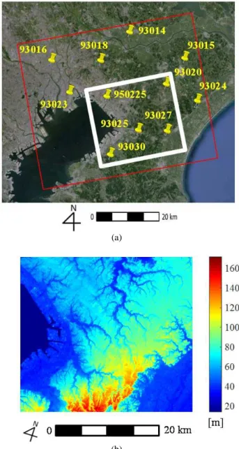
We used 15 SAR images of Chiba Prefecture in Japan that were taken by the Phased Array-type L-band Synthetic Aperture Radar (PALSAR) onboard the Advanced Land Observing Satellite (ALOS). The master and slave images were obtained in Fine Beam Single (FBS) mode (HH polarization) (see Table 1). Figure 1(a) shows the study area. The resolution of these images after multi-looking is 25 m in both the slant range and azimuth directions.
In this study, we use a DEM with a 90-m spatial resolution as obtained by the Shuttle Radar Topography Mission (SRTM), as shown in Figure 1(b). We also use surface temperature and pressure data with a 1-h temporal resolution as forecast by the Research Institute for Sustainable Humanosphere (RISH) of Kyoto University in Japan using a numerical mesoscale model (MSM) (RISH, 2017).
3. PRECIPITABLE WATER
PW is the depth of water contained in a vertical column of unit area from the Earth’s surface to the top of the atmosphere if all that water precipitated as rain. Recently, PW has been identified as radiosonde-measurable meteorological data that can give a direct indication of atmospheric conditions. Specifically, we can calculate PW using observed pressure and specific humidity:
PW , , ⋯ . (1)
Here, is acceleration due to gravity, is surface pressure, is pressure at the ith observational altitude, and , is the mean specific humidity between and .
The atmospheric delay in the zenith direction (∆ ) is calculated as
∆
.
(2)
Here, is surface temperature, is partial pressure of water vapor, is the compression ratio of water vapor, , , are constants, is the gas constant, and and are the molecular weights of dry air and water vapor, respectively. Equation (2) can be divided into a term that is proportional to surface pressure and two terms that are proportional to the amount of water vapor and the temperature, respectively. The first term is known as the zenith hydrostatic delay (ZHD). The other two terms are known collectively as the zenith wet delay (ZWD). Because of its features, ZHD depends on elevation. Therefore, ZHD has little influence on Permanent Scatterers InSAR (PSInSAR) if, in the differential interferogram processing, we use temporal differences between pixels with the same coordinates and elevations. In contrast, ZWD varies considerably between images because the distribution of water vapor depends strongly on time and place. In this study, we improve the accuracy of the interferograms by removing the
ZWD error. The ZWD can be calculated as follows (Askne and Nordius, 1987):
(a)
(b)
Figure 1. Study area. (a) Chiba, near Tokyo, Japan. Red and white rectangles denote areas of PALSAR image and analysis in this research, respectively. Yellow letters denote IDs of GPS base stations, operated by Geography Survey in Japan. (b) DEM derived from SRTM (90-m spatial spacing).
ZWD PW. (3)
4. PROPOSED METHOD
4.1 Estimating PW from meteorological data
We use the 90-m-resolution SRTM DEM data and the 1-h-resolution MSM grid point value (GPV) data to estimate the PW at high spatial and temporal resolutions. The GPV data come in several different types on each pressure isosurface, namely specific humidity (SH), surface temperature ( ), surface pressure ( ), and sea-level surface pressure ( ). The data also comprise the relative humidity (RH) on each pressure isosurface in the range of 300–1000 hPa. These data have spatial resolutions of 0.05°×0.065° at the ground and 0.1°×0.125° on the pressure isosurfaces, and temporal resolutions of 1 h at the ground and 3 h on the pressure isosurfaces (Japan Meteorological Agency, 2017).
The DEM and GPV data are used to estimate PW at each pixel. Because GPV and DEM have different resolutions, we interpolate the GPV resolution to that of DEM. In this subsection, we discuss only a GPV grid and a pixel in the DEM grid. There are u v pixels in , one of which is (i=1,2,..,u; j=1,2,..,v).
Firstly, the surface pressure [hPa] at is estimated. Assuming a temperature lapse rate of 6.5 K/km, the elevation [km] and the sea-level surface temperature _ [K] can be calculated from the equations of state and hydrostatic equilibrium (Equations (4) and (5)):
_
. __
.
, (4)
_ _ . . (5)
Pressure is expressed using and _ :
_
.
_ .
. (6)
Next, we estimate the specific humidity SH . The water vapor pressure hPa] and surface pressure are needed in order to estimate SH . The saturated water vapor pressure
_ hPa] is given by the Tetens equation:
_ . . / . . (7)
Pressure is calculated by using the ratio of to _ to represent the RH:
_
_ . (8)
At pixels that satisfy > 1000 hPa, SH is estimated using the surface and water-vapor pressures:
SH .
. . (9)
Finally, the PW is estimated using and SH . Assuming
RH = RH for > 1000 hPa, is calculated using Equations (5)–(9). Furthermore, for > 1000 hPa, we assume
SH = SH , the latter being the value at the nearest upper pressure isosurface. Between the ground and the 300-hPa isosurface, the PW is given by either Equation (10) or (11). For 1000 hPa, we have
PW ,
⋯
.
(10)
For 1000 hPa, we have
PW SH
SH SH
∙∙
∙ SH SH ;
.
(11)
4.2 Estimating ZWD´ from PW
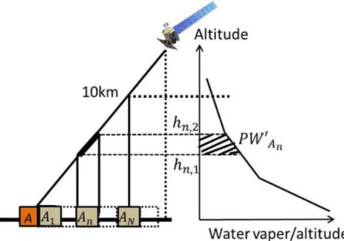
The PW estimated in Subsection 4.1 is that in the zenithal direction. Therefore, when the PW value is entered into Equation (3), only the ZWD in the zenithal direction is estimated. However, in order to remove the atmospheric error correctly, we should integrate the errors along the microwave propagation path. Hereinafter, we use ZWD´ to refer to the integrated ZWD along the slant range direction. In this subsection, we explain the method for estimating ZWD´. Figure 2 shows a flowchart of this process.
For simplicity, we discuss the calculation for a single pixel (pixel A). Firstly, we use orbital information to calculate the incident angle of pixel A and select the pixel group (A1–AN) over which microwaves pass in the range direction. Next, we select only those pixels for which the altitude is less than 10 km because that is where most of the water vapor resides. The altitude is calculated from the incident angle at which microwaves pass above each pixel in the group.
1) Select target pixel A and find pixels A1–AN on the line connecting the target pixel and the sensor
2) Calculate PW on the pressure isosurface of each pixel A1– AN
3) Calculate coefficient from PW = × height
4) Calculate differential PW (PW´) for each pixel by using and height difference h2 – h1
5) Derive cumulative amount of PW´ and convert it into ZWD´.
Figure 2. Estimation of ZWD´ along slant range direction
PW , PW PW . (12)
Here, PW is the PW between the ground and the ith pressure isosurface.
We estimate a coefficient (α) between each pressure isosurface using PW and the altitude difference (∆ ). Thus, the vertical PW can be expressed as a function of altitude at each pixel:
PW ∆ . (13)
In fact, PW´ (the differential PW) influences ZWD´ above each pixel of the group A1–AN. The altitude change above each pixel is calculated from the incident angle and the spatial resolution. Furthermore, PW is calculated using the function between pressure isosurfaces including and :
PW′ , , . (14)
If and exist in different pressure-isosurface intervals, PW´ is calculated instead as:
PW′ , , , , . (15)
Here, is the height of the boundary between the pressure isosurfaces, and is the coefficient of the ith pressure-isosurface interval.
PW′ is the value along the slant range direction and can be estimated by summing up the PW′ values of the group A1–AN:
PW′ PW . (16)
We substitute PW´ into PW in Eq. (3) in order to calculate ZWD´:
ZWD ′ PW ′. (17)
For the interferogram, ZWD´ is acquired by taking the difference between the ZWD´ values of the master and slave images captured at and :
∆ZWD , ZWD ZWD′ . (18)
The phase equivalent to ZWD´ is obtained as
∆ . (19)
4.3 Estimating Phase Delay from ZWD´ and Phase Difference
Figure 3 shows a flowchart of the process for estimating the phase delay. We assume that the interferogram phase delay derived with Equation (19) is mitigated by the SAR image processing (e.g., range migration). Therefore, we assume that the remaining interferogram phase delay ′ can be expressed as a linear function:
′ ⋅ , (20)
where m and n are coefficients.
The atmospheric phase delay is obtained from the interferogram by atmospheric phase screening (APS) estimation, as shown in Figure 3. High-pass temporal and low-pass spatial filters are applied to the residual w derived from a first estimation of the linear displacement velocity and DEM error:
Figure 3. Removal of phase error due to ZWD in the PSInSAR technique.
Assuming that the atmospheric phase delay obtained from the interferogram is equivalent to ′ , m and n are determined by minimizing the sum of the squared residuals between and ′ :
, ≡ , ∑ ∙ . (21)
We determine the residual between and ′ , and subtract it from the original phase difference. Finally, we conduct a second estimation of the linear displacement velocity and DEM error.
5. EXPERIMENT
Figure 4 shows a comparison between the actual and estimated PW. The root mean square error (RMSE) is 3.68 mm. Table 1 lists which SAR images were used for the analysis, and gives the linear-regression coefficients. Figure 5 shows the relationship between and using SAR images 0 and 1 listed in Table 1. The linear regression model so obtained was
= 0.896 – 10.9 for this image pair.
Figure 7 shows the land deformations from September 23, 2006 to January 4, 2011 (i.e., 1564 days) estimated using the proposed method and using the traditional PSInSAR technique
(Ferreti et al. 2000). We coded the PSInSAR processing in MATLAB. The positive and negative deformation values denote uplift and subsidence, respectively. We set GPS station ID 950225 as the reference point from which to calculate the relative deformation. Figure 8 shows the temporal changes of land deformation estimated by the proposed method and by traditional PSInSAR. The results are compared with the temporal change of land deformation observed by GPS. Table 2 gives the RMSEs of land deformation obtained by comparing the deformation via GPS measurements.
Figure 4. Root mean square error (RMSE) of the estimated PW.
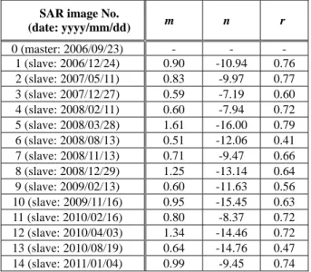
Table 1. SAR images used for the analysis. “m” and “n” denote gain and offset derived by applying a linear regression model (Equation (20)), respectively. “r” denotes correlation coefficient by applying Equation (20).
SAR image No.
(date: yyyy/mm/dd) m n r
0 (master: 2006/09/23) -1 (slave: 2006/-12/24) 0.90 -10.94 0.76 2 (slave: 2007/05/11) 0.83 -9.97 0.77 3 (slave: 2007/12/27) 0.59 -7.19 0.60 4 (slave: 2008/02/11) 0.60 -7.94 0.72 5 (slave: 2008/03/28) 1.61 -16.00 0.79 6 (slave: 2008/08/13) 0.51 -12.06 0.41 7 (slave: 2008/11/13) 0.71 -9.47 0.66 8 (slave: 2008/12/29) 1.25 -13.14 0.64 9 (slave: 2009/02/13) 0.60 -11.63 0.56 10 (slave: 2009/11/16) 0.95 -15.45 0.63 11 (slave: 2010/02/16) 0.80 -8.37 0.72 12 (slave: 2010/04/03) 1.34 -14.46 0.72 13 (slave: 2010/08/19) 0.64 -14.76 0.47 14 (slave: 2011/01/04) 0.99 -9.45 0.74
Estim
ated PW (m
m
Figure 5. Example of scattergram between ZWD phase and atmospheric phase delay by using images 0 and 1 listed in Table 1.
Figure 6. Estimated ZWD´ phase for the interferogram of images 0 and 1.
6. DISCUSSION
Firstly, we discuss the methodology for estimating the atmospheric phase delay from external meteorological data. As shown in Figure 4, the RMSE of the estimated PW, 3.68 mm, is acceptable for use in removing the atmospheric phase delay from the interferogram phase. It was confirmed that the interpolation of PW was successful. Figure 5 indicates that there is a positive correlation between and . The mean of the correlation coefficients derived from Table 1 was 0.66. This indicates that the approach of removing the ZWD´ contribution to the phase in order to improve the land-deformation accuracy is reasonable.
Next, we address the issue of the relatively low mean of the correlation coefficients. We applied high-pass temporal and
low-pass spatial filters to the residual derived from a first estimation of the linear displacement velocity and DEM error. This filtering may have removed only the atmospheric delay from , and should be investigated further.
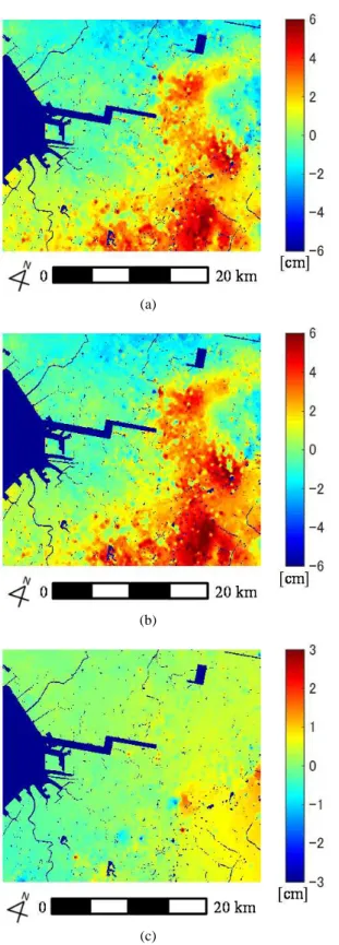
Finally, we focus on the improvement of land-deformation accuracy by PSInSAR. In the lower right of Figures 7(a) and 7(b), a large subsidence is estimated. This result is consistent with the field survey conducted by the Chiba Prefectural Government, Japan (Chiba Prefectural Government, 2017). Figure 7(c) shows that the main differences between the results using traditional PSInSAR (Figure 7(a)) and those using the proposed method (Figure 7(b)) are limited to the lower right of the study area. There is no noticeable deformation at GPS ID93025 (Figure 8(a)), whereas there is an almost linear subsidence velocity at GPS ID93027. As given in Table 2, there is no significant improvement in the RMSE of the estimated land deformation at ID93025, whereas the RMSE was improved at ID93027. In addition, the land-deformation RMSE at ID93020 remains the largest among the four GPS stations. This can be explained by the fact that there are far fewer permanent scatters (PSs) in the area around this station than around the other stations. Hence, the network connecting the PSs may not reflect the local land deformation. This issue is often the case with the PSInSAR technique, and it may be necessary to adopt a different approach to detecting distributed scatterers (DSs).
7. CONCLUSIONS
In this paper, we presented a method for mitigating the atmospheric phase delay by using external meteorological data to improve the accuracy of land-deformation assessment using the DInSAR technique. The proposed method calculates and interpolates the PW with regard to the spatial and temporal resolutions.
We then derived the cumulative amount of differential PW at the height of the slant range vector at pixels along that direction. The atmospheric phase delay of each interferogram was acquired by taking a residual after a preliminary determination of the linear deformation velocity and DEM error, and by applying high-pass temporal and low-pass spatial filters. Next, we estimated a regression model between the cumulative amount of PW and the atmospheric phase delay. Finally, we subtracted the contribution of the atmospheric phase delay from the phase difference of the interferogram, and determined the linear deformation velocity and DEM error.
(a)
(b)
(c)
Figure 7. Contrasting results using the traditional PSInSAR technique and those using the proposed method: (a) deformation derived using traditional PSInSAR (Ferreti et al., 2000); (b) deformation derived using proposed method; (c) difference between (a) and (b). Positive and negative deformation values denote uplift and subsidence, respectively.
(a)
(b)
Figure 8. Land deformation estimated using the proposed method: (a) GPS station ID 93025; (b) ID 93027.
Table 2. RMSEs of land deformation of GPS stations
GPS Station ID
RMSE (cm)
Traditional PSInSAR Proposed method
93020 1.57 1.46
93025 0.77 0.71
93027 1.12 0.88
93030 0.69 0.64
REFERENCES
Akatsuka, S., Oyoshi, K., and Takeuchi, W., 2013. Development of an Optimum Water Vapor Product for Land Surface Temperature Retrieval from MTSAT data. Journal of The Remote Sensing Society of Japan, 33(3), pp. 173-184.
Alshawaf, F., Fuhrmann, T., Knöpfler, A., Luo, X., Mayer, M.,
de
fo
rm
ation (m
m
Hinz, S. and Heck, B. 2015. Accurate estimation of atmospheric water vapor using GNSS observations and surface meteorological data. IEEE Transactions on Geoscience and Remote Sensing, Vol. 53, No. 7, pp. 3764-3771.
Askne, J., and Nordius, J., 1987, Estimation of tropospheric delay for microwaves from surface weather data, Radio Science, 22, 379-386.
Beivis, M., Businger, S., Herring, T.A., Rocken, C., Anthes, R.A. and Ware, R.H., 1992. GPS meteorology : Remote sensing of atmospheric water vapor using the global positioning system, Journal of Geophysical Research, vol. 97, no. D14, pp. 15787-15801.
Berardino, P., Fornaro, G. Lanari, R. and Sansosti, E., 2002. A new algorithm for surface deformation monitoring based on small baseline differential SAR interferograms, IEEE Trans. Geosci. Remote Sens., vol. 40, no. 11, 2002.
Chiba Prefectural Government, 2017. Current status of land subsidence in Chiba Prefecture. https://www.pref.chiba.lg.jp/ suiho/jibanchinka/torikumi/genkyou.html (in Japanese) (accessed on Feb. 23, 2017).
Davies, O.T. and Watson, P.A., 1999. GPS phase-delay measurement: Technique for the calibration and analysis in millimeter-wave radio propagation studies. IEE Proc. Microwa. Antennas Propag., vol. 146, no. 6, pp.369-373.
Ferretti, A., Prati, C. and Rocca, F., 2000. Nonlinear subsidence rate estimation using permanent scatterers in differential SAR interferometry, IEEE Trans. Geosci. Remote Sens., vol. 38, no. 5, 2000.
Ferretti, A., Prati, C., and Rocca, F., 2002. Nonlinear subsidence rate estimation using permanent scatterers in differential SAR
interferometry. IEEE Transactions on Geoscience and Remote Sensing, 38(5), pp. 2202-2212.
Fujiwara, S., Tobita, M., Murakami, M., Nakagawa, H., and Rosen, A., P., 1999. Baseline Determination and Correction of Atmospheric Delay Induced by Topography of SAR Interferometry for Precise Surface Change Detection. Journal of the Geodetic Society of Japan, 45(4), pp. 315-325.
Japan Meteorological Agency, 2017. Technical report No. 205, http://www.data.jma.go.jp/add/suishin/jyouhou/pdf/205. pdf (accessed on Feb. 23, 2017).
Kampes, B. M., 2006. Radar Interferometry. Springer Netherlands, pp. 5-30.
Li, Z., Fielding, E.J. and Cross, P. 2009. Integration of InSAR time-series analysis and water-vapor correction for mapping postseismic motion after the 2003 Bam (Iran) Earthquake. IEEE Transactions on Geoscience and Remote Sensing, Vol. 47, No. 9, pp. 3220-3230.
Mateus, P., Nico, G. and Catalão, J., 2014. Maps of PWV temporal changes by SAR interferometry: A study on the properties of atmosphere’s temperature profiles. IEEE Geoscience and Remote Sensing Letters, Vol. 11, No. 12, pp. 2065 - 2069
Ohtani, R., Tsuji, H., Mannoji, N., Segawa, J. and Naito, I., 1997. Precipitable Water Vapor Observed by Geographical Survey Institute’s GPS Network. Meteorological Society of Japan, Tenki 44(5), pp. 317-325.