Jörg Menche max struc pre 2010

Asymptotic properties of degree-correlated scale-free networks

Jörg Menche, Angelo Valleriani, and Reinhard Lipowsky

Max-Planck-Institute of Colloids and Interfaces, Science Park Golm, 14424 Potsdam, Germany 共Received 23 October 2009; published 9 April 2010兲

The possible correlation profiles of networks with a given scale-free degree distribution are restricted and bounded by maximallycorrelated configurations.Dissortativenetworks consist of nested bilayers, in which low-degree vertices are connected to high-degree vertices. The number of these bilayers attains a constant value for large network sizeN.Assortativenetworks exhibit monolayers of low-degree vertices, the number of which grows monotonously with N. Analytical relations for the Pearson correlation coefficient r of these extremal configurations are derived and shown to provide lower and upper bounds on the possiblervalues. Both bounds are found to vanish for large networks.

DOI:10.1103/PhysRevE.81.046103 PACS number共s兲: 89.75.Fb, 05.50.⫹q

I. INTRODUCTION

In recent years, many real world systems have been suc-cessfully described as complex networks 关1–3兴. Especially scale-free networks, in which the probabilityP共k兲of finding a vertex withkneighbors decays as a power law P共k兲 ⬃k−␥

have been studied intensively. Generally, the degree distribu-tion alone does not suffice to completely describe the inner structure of a given network. An important additional mea-sure is given by the so-called assortativity by degree 关4,5兴, which quantifies the tendency of vertices to be connected to other vertices of similar degree. Networks areassortativeif vertices with high degree preferably connect to other vertices with high degree. Networks aredissortativeif vertices with high degree are linked to vertices with low degree. Technical and biological networks have been found to be dissortatively mixed, while social networks show assortative correlations 共see关2,4,5兴for detailed lists兲.

Degree correlations play an important role for many struc-tural properties of networks, e.g., percolation thresholds 关4,6,7兴, mean distance关6,7兴, or robustness against vertex re-moval 关4,5,8兴. Likewise, they also affect the properties of dynamical processes taking place on networks, such as epi-demic spreading关9–11兴, stability against stimuli and pertur-bation 关12,13兴, or synchronization of oscillators关14,15兴.

In this paper, we analyze in detail a class of maximally

correlated scale-free networks. These networks provide valu-able limiting cases for all possible correlation profiles of net-works with scale-free degree distributions. We provide an analytical description in terms of the most commonly used measures of assortativity. In particular, we give asymptotic boundary values for the range of all possible values of the

Pearsoncorrelation coefficient, which is found to vanish for

large networks.

Further, we give an intuitive characterization of maxi-mally correlated networks in terms of layers of vertices of the same degree. We find a pronounced community structure that can be useful for the understanding of various phenom-ena taking place on scale-free networks.

Our paper is organized as follows: in Sec.II, we introduce the basic parameters of our system, discuss the different measures of assortativity, and review the algorithm from 关6,7兴that we use to construct maximally correlated networks.

We then analyze the structural properties of 共i兲 maximally dissortative and 共ii兲 maximally assortative networks before we close with a brief discussion and summary.

II. MODELS AND METHODS

We use scale-free networks with a fixed degree distribu-tion given by

P共k兲= 1

Ak

−␥ _{for k}

0ⱕkⱕkmax

= 0 otherwise, 共1兲

where A_{denotes the normalization constant. The structural} parameters of our networks are the number of verticesN, the exponent ␥, and the minimal degree k0. In this work, we focus on the range 2⬍␥⬍3, which applies to most real world networks. Further, we consider only simple networks without multiple connections or self-loops 关29兴. For the maximal degree kmax, we use the so-called natural cutoff 关16兴

k_max=k₀N1/共␥−1兲_{. 共2兲}

A combination of the two relations 共1兲and 共2兲 leads to the normalization constant

A₌

兺

k=k₀ k_max

k−␥⬇

冕

k₀ k_max

k−␥dk= 1

␥− 1k0 1−␥

冉

1 − 1

N

冊

. 共3兲

Depending on the parameters ␥ and k0, there is a certain network size, below whichkmaxexceedsN. In the latter case, we usekmax=N− 1, so that the maximal degree can be written as

kmax= min共k0N1

/共␥−1兲_{,N− 1兲 共4兲}

for all values ofN. The natural cutoff follows from the well-known configuration model关17兴that we use to generate the networks for our simulations. Many structural properties of scale-free networks depend on the scaling of kmax with N, such as the probability of multiple links and self-loops 关18兴 or clustering 关19兴. As discussed in detail in 关18,20,21兴, the cutoff also plays an important role for the construction of scale-free networks with a given correlation profile. As

tioned before, we consider the opposite case: We take the degree distribution as fixed and study the subsequent con-straints on the maximaldegree correlations. The qualitative results presented below do not depend on the choice of the maximal degree, while the analytical calculations can easily be adapted to other choices of kmax.

A. Measures of assortativity

A complete description of the degree correlations within a network is provided by the joint probability P共j,k兲 that a randomly chosen link connects two vertices of degree j and

k. This quantity has been used in关22,23兴to study the corre-lations in protein interaction networks and the internet. The interpretation of P共j,k兲 is often difficult because of large statistical fluctuations that occur especially for high degrees. As a more robust measure the average degree

Knn共k兲 ⬅

兺

j

jP共j兩k兲 共5兲

of the neighbors of a randomly chosen vertex of degree k

was introduced in 关24,25兴, where P共j兩k兲 denotes the condi-tional probability that the neighbor of a vertex with degreek

has degree j. The conditional probabilityP共j兩k兲is related to the joint probability P共j,k兲via

P共j兩k兲=P共j,k兲

PM共k兲

, 共6兲

wherePM共k兲is the probability to find a vertex of degreekat

the end of a randomly chosen edge with

PM共k兲=

P共k兲k

兺

k_⬘=k₀ k_max

P共k

_⬘

兲k

_⬘

= P共k兲k 具k典N

. 共7兲

Here and below, the index N of 具·典N indicates an average

over allNvertices. Inuncorrelatednetworks, the degrees of two neighboring vertices are statistically independent, so the joint probability factorizes as Pu_共j,k兲=P

M共j兲PM共k兲 and

P共j兩k兲is identical to the probabilityP_M共j兲. Inserting Eq.共7兲 in Eq.共5兲leads to

K_nnu 共k兲 ⬅K_nnu ⬅

兺

j

j jP共j兲 具k典N

=具k 2_典

N

具k典N

, 共8兲

i.e., Knn does not depend on k in networks without degree correlations. Assortatively mixed networks are associated with an increase inKnnas a function ofk, while dissortative networks show a decrease inKnnas kincreases.

An even more compact and widely used measure for as-sortativity has been introduced in关4,5兴. The assortativity of a given network is measured by a single scalar parameterrthat is basically the Pearsoncorrelation coefficient

r⬅

兺

j,k

jk关P共j,k兲−PM共j兲PM共k兲兴

␴M,j␴M,k

. 共9兲

for the degreesj andkof the two vertices on both ends of a randomly chosen edge 关30兴. The correlation coefficient is

normalized by the standard deviations ␴M,j⬅

冑

具j2典M−具j典M

2

and␴M,k⬅

冑

具k2典M−具k典M

2

, such that its value lies in the range −1ⱕrⱕ1. Note that the index M of具·典Mindicates an

aver-age over allM edges in the network. From Eq.共9兲it is easy to see that uncorrelated networks, with P共j,k兲=Pu_共j,k兲 =PM共j兲PM共k兲 are characterized by a vanishing correlation

coefficientr= 0. A positive correlation coefficientr⬎0 indi-cates assortative mixing, negative values likewise dissorta-tive correlations. However, as we will show below, this dis-tinction can be misleading for networks with broad degree distributions and should be checked carefully.

B. Rewiring procedure for maximal correlations There is a variety of algorithms available in order to con-struct correlated networks. In Refs.关5,21,26兴, different meth-ods are introduced, for which both the degree distribution

and the correlation structure are given. Such algorithms are especially useful for the analysis of real world networks, where null models are needed that conserve certain statistical properties, but are otherwise as uncorrelated as possible. In this paper, we follow a somewhat complementary approach. We study the constraints that a prescribed degree distribution of a network poses on its possible degree correlations. We therefore use a rewiring algorithm from Refs. 关6,7兴 that al-lows for the construction of maximally correlated configura-tions for a given network with fixed degree sequence. In each step of the iterative algorithm, two edges with four vertices at their ends are chosen at random. Now, we label these vertices witha,b,c, andd such that their degreeska,kb,kc,

andkdare ordered as

kaⱖkbⱖkcⱖkd. 共10兲

Breaking of the two edges and rewiring of the vertices to form pairsa,b andc,dleads to assortative networks, while connecting a with d andb withc leads to dissortative net-works. For simple networks, we check during an additional step, whether the new connections are allowed and return to the previous configuration otherwise.

The networks that are obtained after iteration of this pro-cedure are maximally assortative or dissortative both in an intuitive fashion as well as in the sense that the Pearson

coefficient attains its maximal or minimal valuermaxorrmin, respectively. To show this, we rewrite definition 共9兲of ras

r=具jk典M−具j典M具k典M

␴M,j␴M,k

共11兲

=

兺

m=1

M

jmkm−

1

M

冉

m

兺

=1

M

km

冊

2

兺

m=1

M

k_m2 − 1

M

冉

m

兺

=1

M

km

冊

2 . 共12兲

兺

m=1

M

km=

兺

k=k₀ k_max

NP共k兲k2=N具k2典N, 共13兲

兺

m=1

M

k_m2 =

兺

k=k₀ k_max

NP共k兲k3=N具k3典N. 共14兲

Using Eqs. 共13兲 and 共14兲, we can rewrite r in Eq. 共12兲 in terms of the moments of the degree distribution, which leads to

r⬅Ar−Br

Cr−Br

, 共15兲

with

Ar⬅

兺

m=1

M

jmkm, 共16兲

Br⬅

N2

M具k

2_典

N

2

, 共17兲

and

Cr⬅N具k3典N. 共18兲

Since the degree distributionP共k兲is fixed, bothB_randC_rare fixed as well and do not change as one rewires the network. The only term that is affected by this rewiring isAras given

by Eq. 共16兲, which enters the numerator of Eq. 共15兲. There are only three possibilities to distribute two edges between four vertices, which lead to the terms

kakb+kckd, 共19兲

k_ak_d+k_bk_c, 共20兲

kakc+kbkd 共21兲

inAr. These terms satisfy the relations

kakd+kbkc=kakc+kbkd−共ka−kb兲共kc−kd兲, 共22兲

kakc+kbkd=kakb+kckd−共ka−kd兲共kb−kc兲. 共23兲

It now follows from these two relations together with Eq. 共10兲that

kakd+kbkcⱕkakc+kbkdⱕkakb+kckd. 共24兲

Therefore, configuration共19兲gives the biggest and configu-ration 共20兲 the smallest contribution to Ar and, thus, to r.

These are exactly the chosen configurations in the two ver-sions of the algorithm, so successive iteration of these choices will eventually lead to an asymptotic network with maximal degree correlations, whererattains its maximal and minimal values rmax and rmin respectively. In general, it is possible that such a simple “hill climbing” algorithm be-comes trapped in local minima. We therefore checked very carefully that this is not the case in this system. First, we performed several realizations of the random search path starting from the same initial network, each with O共M2_兲

it-eration steps. When we compare the resulting networks, we find that all properties discussed below are preserved across all final network configurations. Second, in analogy with simulated annealing, i.e., with increasing the temperature in order to overcome local energy barriers, we allowed for ran-dom rewiring with a certain probability p in each iteration step. Starting from completely random rewiring with p= 1 and decreasing the “temperature” stepwise top= 0, we again converge to the same final configurations as before.

In the following sections, we will analyze the structure of such networks in detail and give analytical expressions for

rmin andrmax. We begin with a discussion of maximally dis-sortative networks.

III. MAXIMALLY DISSORTATIVE NETWORKS A. Structural properties

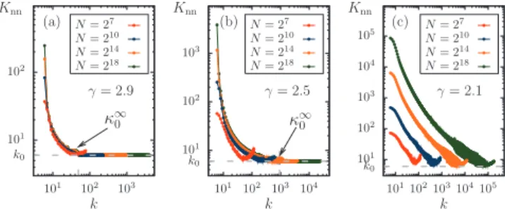
Figure 1 shows the average nearest-neighbor degree

Knn共k兲for maximally dissortative networks for different net-work sizes N and decay exponent␥. All curves exhibit the expected decrease of Knn with increasingk, only for largek some curves show a small increase inK_nn共k兲. The respective vertices have so many edges that they cannot be saturated with low-degree vertices alone so that they connect also to some vertices with a higher degree. This effect is more pro-nounced for networks with small N and small exponent ␥. For sufficiently largeNand␥, we find the high-degree region

kⱖ␬0 for which Knn共k兲 ⯝k0, i.e., all vertices with degreek

ⱖ␬0 are predominantly connected to k0 vertices. Close in-spection of Figs.1共a兲and1共b兲reveals that for large networks the value of␬0 does not depend onN.

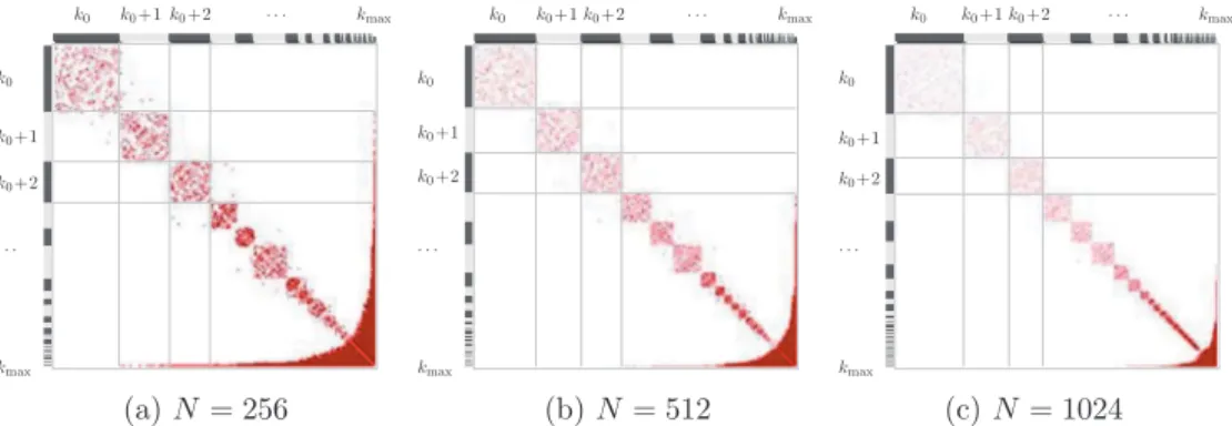
For a more detailed analysis of the structure of these net-works, we consider the adjacency matrix A, which has N ⫻N entries Aij with Aij= 1 if the vertices i and j are

con-nected andAij= 0 otherwise. When the indices are rearranged

according to the degree of the vertices, one can clearly iden-tify distinct rectangular patterns of connected vertices 共see Fig.2兲. These patterns correspond to nested bilayers, where vertices with low degree are connected to vertices with high degree. Since the adjacency matrix is symmetric with Aji

=A_ij, the “necklace” contains a central cluster with degree

k0

101

102

101

102

103

Knn

k

κ∞

0

N= 218

N= 214

N= 210

N= 27

k0

101

102

103

101

102

103

104

Knn

k

κ∞

0

N= 218

N= 214

N= 210

N= 27

k0

101

102

103

104

105

101

102

103

104

105

Knn

k

N= 218

N= 214

N= 210

N= 27

(a) (b) (c)

γ= 2.9 γ= 2.5 γ= 2.1

FIG. 1.共Color兲Average degreeKnnof the nearest neighbors of a

randomly picked vertex with degree k for maximally dissortative networks with different sizes N and exponent 共a兲 ␥= 2.9, 共b兲 ␥

= 2.5, and 共c兲 ␥= 2.1. All curves are averages over 100 networks withk0= 6. Sufficiently large networks in共a兲and共b兲show a plateau

with kⱖ␬0 for which Knn共k兲=k0. The asymptotic values ␬0⬁ as

kme. On the low-degree side, the vertices are characterized by a single degreekn⬍kme, the vertices on the high-degree side

have degrees in between the boundary values ␬nⱗkⱗ␬n−1. The outermost bilayer consists of thek0vertices that connect to all vertices with␬0ⱗkⱕkmax, which leads to the region of

Knn共kⲏ␬0兲 ⯝k0 that can be identified in Fig.1. The second bilayer contains all vertices withk0+ 1 on the one side and all vertices with␬1ⱗkⱗ␬0 on the other side, the third one all vertices with k0+ 2 and ␬2ⱗkⱗ␬1, and so forth. The total number of bilayers is limited by the central cluster of kme vertices, around which they are nested共see Fig.2兲. Note that in principle, network realizations might be generated, in which some of the bilayers disconnect completely from the rest of the network. However, in practice, in our simulations we find that the corresponding degree sequences, for which the numbers of edges on both sides of a bilayer match

ex-actly, are extremely unlikely to occur关31兴.

In addition to the necklace of clusters, we find for small networks as in Figs. 2共a兲and2共b兲that the last row and col-umn, which represent thekmaxvertices, are connected to sev-eral low-degree layers, corresponding to the increase in Knn for large degrees in Fig.1.

In the following, we will consider these effects in more detail and begin with the influence of the kmax vertex. It follows from the expression in Eq.共4兲that the upper cutoff is given bykmax=N− 1 for

N⬍N₁⬅k₀共␥−1兲/共␥−2兲, 共25兲

so vertices with degree kmax are connected to all remaining vertices in the network. ForN⬎N1, thekmaxvertex no longer spans the entire network but is still connected to all vertices withk₀ⱕkⱕk_A. The value ofk_Acan be determined from the relation

kmax=

兺

k=k₀ k_A

Nk⬇

冕

k₀ k_A

NP共k兲dk= 1

1 −␥ N

A共kA 1−␥

−k₀1−␥兲,

共26兲

whereNkdenotes the number of vertices with degreek.

Solv-ing Eq. 共26兲fork_Aleads to

kA=k0

冋

1 −

冉

1 −

1

N

冊

k0N

共2−␥兲/共␥−1兲

册

1/共1−␥兲

. 共27兲

For N= 256, ␥= 2.9, and k0= 6, relation 共27兲 gives kA⯝8, which agrees well with Fig.2共a兲, where thekmaxvertex pro-trudes into the layer of k= 8. In the limit of large networks with NⰇN1, expression 共27兲 behaves as kA⬇k0, and all edges of thekmaxvertex are saturated byk0vertices关see Fig. 2共c兲兴. As we have seen above, thek0 vertices are numerous enough to saturate all vertices with degree kⱖ␬0, which leads to the formation of the outermost bilayer. The value of

␬0can be obtained from

Nk₀k0=

兺

k=␬0

k_max

Nkk, 共28兲

or

NP共k₀兲k₀=

兺

k=␬0

k_max

NP共k兲k⬇

冕

␬0

k_max

NP共k兲kdk

= 1

2 −␥ N

A共kmax 2−␥

−␬0

2−␥_{兲. 共29兲}

Solving Eq.共29兲for ␬0 leads to

␬0=k0

冉

␥− 2

k₀ +N

共2−␥兲/共␥−1兲

冊

1/共2−␥兲

. 共30兲

For large networks with

NⰇN2⬅

冉

k0

␥− 2

冊

共␥−1兲/共␥−2兲

, 共31兲

the degree ␬0 attains the constant value

␬0⬇␬0 ⬁

⬅k₀共␥−1兲/共␥−2兲共␥− 2兲1/_共2−␥兲_{. 共32兲}

This behavior can be seen in Figs.1共a兲and1共b兲, where the values of␬0

⬁

as obtained from Eq. 共32兲 are indicated. For␥

= 2.1 as in Fig.1共c兲the value ofN₂as defined by Eq.共31兲is given byN2⯝3.6⫻1019⬎264, so the depicted network sizes are too small to observe the plateau behavior.

kme

kme

κ0

κ0

κ1

κ1

kmax

kmax

k0

k0

k1

k1

k2

k2

· · ·

· · · · · ·

kme

kme

κ0

κ0

κ1

κ1

kmax

kmax

k0

k0

k1

k1

k2

k2

· · ·

· · · · · ·

kme

kme

κ0

κ0

κ1

κ1

kmax

kmax

k0

k0

k1

k1

k2

k2

· · · · · ·

· · ·

(a)N _{= 256 (b)}N _{= 512 (c)}N _{= 1024}

FIG. 2. 共Color兲Adjacency matrix Afor three maximally dissortative networks with␥= 2.9,k0= 6 and different sizes 共a兲 N= 256,共b兲

N= 512, and共c兲N= 1024. The vertices are arranged according to their degree, starting with thek₀vertices at the upper left corner to thek_max

Using expression 共32兲 for␬0, we can also determine the values of the degrees ␬n that determine the borders of the

large degree side of the bilayers. As in Eq.共28兲, the degree

␬1can be computed by

Nk₀+1共k0+ 1兲=

兺

k=␬1

␬₀

Nkk, 共33兲

the higher values␬2,␬3, . . . then follow from iteration of Eq. 共33兲with the respective limits in the summation. As we have seen in Fig.2, the series of bilayers is limited by the central degree kme. The value of kme can be determined using the condition that the number of edges attached to all vertices withk⬍kme is equal to the number of edges attached to all vertices withk⬎kme. Solving the implicit equation

兺

k=k₀ k_me

Nkk=

兺

k=k_me k_max

Nkk, 共34兲

we obtain

kme= 21

/共␥−2兲_{k0共1 +N}共2−␥兲/共␥−1兲_兲1/共2−␥兲

. 共35兲

This expression becomes independent of N in the limit of large networks and attains the asymptotic value

kme⬇kme

⬁ _⬅

21/共␥−2兲_k

0. 共36兲

The number Nbiof bilayers as given bykme−k0 is therefore limited and reaches

Nbiⱕmax共Nbi兲=kme

⬁

−k0 共37兲

for large networks.

B. Scaling relation forrmin

After the detailed description of the layered structure of maximally dissortative networks, we will now discuss asymptotic estimates for the corresponding minimal assorta-tivity coefficient r=rmin. We start from the general expres-sion as given by Eq.共15兲. As we have seen before, the only term that depends on the degree correlation isAras given by

Eq. 共16兲; minimal assortativity rmin can therefore be ex-pressed as

r_min=min共Ar兲−Br

C_r−B_r . 共38兲

In the following, we will first determine the asymptotic be-havior ofB_randC_ras given by Eqs.共17兲and共18兲and then address the scaling behavior of min共Ar兲. We start with the

total number of edgesM, which can be obtained from

M=N具k典N=N

兺

k=k₀ k_max

P共k兲k= N A_k

兺

_=k

0

k_max

k1−␥⬇ N

A

冕

_k

0

k_max

k1−␥dk

= ␥− 1

␥− 2Nk0

1 −N共2−␥兲/共␥−1兲

1 − 1

N

. 共39兲

The moments of degree distribution 共1兲 have the general form

具kn典N=

兺

k=k₀ k_max

P共k兲kn⬇

冕

k₀ k_max

P共k兲kndk

=k0

n ␥− 1

n+ 1 −␥

1

1 − 1

N

共N共n+1−␥兲/共␥−1兲− 1兲. 共40兲

It now follows from expressions 共39兲and 共40兲for the total edge number M and the second moment 具k2_典

Nthat the term

B_ras defined in Eq. 共17兲scales as

Br⬃k0

3_N3/共␥−1兲 _{for 1⬍␥⬍2 共41兲}

⬃k₀3N共5−␥兲/共␥−1兲 for 2⬍␥⬍3 共42兲

⬃k₀3N for 3⬍␥ 共43兲

in the limit of largeN. Likewise, the large-Nbehavior of the term Cris given by

Cr⬃k0

3

N3/共␥−1兲 for 1⬍␥⬍4 共44兲

⬃k₀3N for 4⬍␥, 共45兲

as follows from expression 共40兲for the third moment具k3_典

N.

Finally, we now derive the scaling behavior of min共A_r兲. In order to do so, it is convenient to assign an arbitrary but fixed direction to each edgem, such that it emanates from a vertex with degree jmand points at a vertex with degreekm. Now

we label the edges in such a way that the degrees of the vertices they point at increase, i.e.,

k1ⱕk2ⱕ ¯ ⱕkM. 共46兲

In dissortative networks, low-degree vertices are connected to high-degree vertices. The smallest value of Aris then

ob-tained in a configuration, where the degrees of the vertices, from which the edges in Eq. 共46兲 emanate, decrease. This corresponds to

jm=Jm⬅kM−m 共47兲

so that the sequence of J1,J2, . . . ,J_Msatisfies accordingly

J1ⱖJ2ⱖ ¯ ⱖJM. 共48兲

When self- and multiple connections are allowed, it is al-ways possible to rewire a given network such that Eqs. 共46兲–共48兲are fulfilled. However, in dissortatively mixed net-works multiple edges do not play an important role anyway, because these networks contain many vertices with small de-grees that can be connected to the few hubs, and multiple connections can therefore be avoided. In the limit of large networks, the fraction of multiple edges vanishes, so we can use Eqs. 共46兲–共48兲 also for simple networks. The choice in Eq. 共47兲leads to

min共Ar兲=

兺

m=1

M

kmJm=

兺

m=1

M

kmkM−m. 共49兲

Since the termkmkM−mdoes not change when we substitute

min共Ar兲= 2

兺

m=M/2

M

kmJm= 2

兺

m=M/2

M

kmkM−m. 共50兲

From the ordering of the factorsJmin Eq.共48兲we can derive

the following inequalities:

JM/2=kM/2ⱖJmⱖJM=k0 for M/2ⱕmⱕM.

共51兲

When these inequalities are used in expression 共50兲 for min共Ar兲, we obtain both an upper and a lower bound for

min共A_r兲as given by

2kM/2

兺

m=M/2

M

kmⱖmin共Ar兲ⱖ2k0

兺

m=M/2

M

km. 共52兲

By construction, the value of k_M/2 is given by the central degree kme in Eq. 共35兲, for which the vertices with degree

k⬍kmehave the same number of edges as the vertices with

k⬎kme. For largeN, relation共35兲implies the scaling behav-ior

kme⬇21

/共␥−2兲_k

0N1

/共␥−1兲 _{for 1⬍␥⬍2 共53兲}

⬇21/共␥−2兲_k

0 for 2⬍␥. 共54兲

The sum over M/_{2 edges in Eq.} 共₅₂兲 _{can again be} trans-formed into a sum over all degrees,

兺

m=M/2

M

km=

兺

k=k_me k_max

NP共k兲k2⬇

冕

k_me k_max

NP共k兲k2dk

= N A

1 3 −␥共kmax

3−␥

−k_me2−␥兲, 共55兲

together with the asymptotic behavior ofk_mein Eq.共54兲we find

兺

m=M/2

M

km⬃k0

2

N2/共␥−1兲 for 1⬍␥⬍3 共56兲

⬃k0N for 3⬍␥. 共57兲

We now combine the asymptotic behavior of k_me and 兺m=M/2

M _k

mas given by Eqs.共53兲,共54兲,共56兲, and共57兲with the

two inequalities contained in Eq. 共52兲. First, we insert Eqs. 共53兲and共56兲into Eq.共52兲and obtain

c1k0 3

N3/共␥−1兲ⱖmin共Ar兲ⱖc2k0 3

N2/共␥−1兲 共58兲

for 1⬍␥⬍2 with two␥-dependent constantsc1andc2. This implies the asymptotic behavior of min共Ar兲 as given by

min共Ar兲 ⬃k0 3

N␨ for 1⬍␥⬍2 共59兲

for largeN where the exponent␨satisfies the inequalities 2

␥− 1ⱕ␨ⱕ 3

␥− 1. 共60兲

Second, we use the asymptotic behavior in Eqs. 共54兲 and 共56兲together with the inequalities共52兲to obtain

c₁

_⬘

k₀3N2/共␥−1兲_ⱖmin共A

r兲ⱖc2k0

3_N2/共␥−1兲 _共61兲

for 2⬍␥⬍3, which leads to min共Ar兲 ⬃k0

3

N2/共␥−1兲 for 2⬍␥⬍3. 共62兲

For the region ␥⬎3, we combine the two asymptotic rela-tions共54兲and共57兲with the inequalities共52兲and obtain

min共Ar兲 ⬃k0 3_N

for 3⬍␥. 共63兲

Putting the relations for min共Ar兲 as given by Eqs.

共59兲–共63兲 together withB_r andC_r in Eqs. 共41兲–共45兲 we fi-nally arrive at a general expression for the scaling behavior of the Pearson coefficient for maximally dissortative net-works:

rmin⬃−c1共␥,k0兲 for ␥⬍2

⬃−N共2−␥兲/共␥−1兲 for 2⬍␥⬍3 ⬃−N共␥−4兲/共␥−1兲 for 3⬍␥⬍4

⬃−c2共␥,k0兲 for 4⬍␥, 共64兲

with the two ␥- and k0-dependent constants c1 and c2. For 2⬍␥⬍3 the same result has also been derived in关27兴.

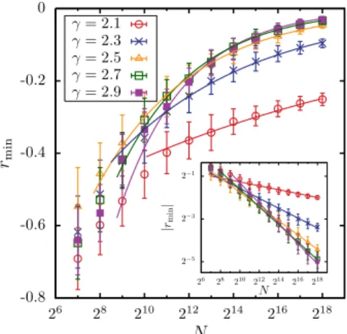
For 2⬍␥⬍4 it follows from Eq.共64兲that the correlation coefficient vanishes in the limit of large N, which is con-firmed by simulations 共see Fig. 3兲. This is surprising since the structure of the underlying networks is nevertheless highly correlated, as we have seen in the previous section. We conclude that while uncorrelated networks are charac-terized by a vanishing correlation coefficient, the opposite is not necessarily true. Especially for large networks, the

Pearson coefficient is not sufficient to judge the correlation

-0.8 -0.6 -0.4 -0.2 0

26

28

210

212

214

216

218

rmin

N

γ= 2.1

γ= 2.3 γ= 2.5

γ= 2.7 γ= 2.9

2−5

2−3

2−1

26 28 210 212 214 216 218

|

rmin

|

N

FIG. 3. 共Color online兲 Pearsoncoefficientrmin for maximally

dissortative networks as a function of network sizeNfor different values of the scaling exponent␥. All data points are averages over 100 networks with minimal degreek0= 6, error bars denote the

stan-dard deviation. The lines are fits using Eq.共64兲with the amplitude as the only fit parameter. For all values of the exponent␥, the data for the minimalPearsoncoefficientrmindecay to zero for largeN,

in good agreement with the theoretical predictions. The inset shows the same data for兩rmin兩as a function of Nin a double-logarithmic

structure of a given network, and additional measures need to be taken into account.

IV. MAXIMALLY ASSORTATIVE NETWORKS

We will now turn to maximally assortative networks, starting with a discussion of their main structural character-istics.

A. Structural properties

For a first overview, we consider again the adjacency ma-trixA共see Fig.4兲. Using the previously explained ordering according to the degree of the vertices, we find pronounced quadratic regions in A. These regions represent monolayers of vertices, which are only connected to vertices of the same degree. A comparison of Figs.4共a兲–4共c兲shows that the num-ber of such layers grows with network sizeN. Furthermore, inspection of these figures also reveals a region of high-degree vertices with kⱗkmax, the edges of which span sev-eral layers of vertices and thereby limit the number of low-degree vertices that are connected only to vertices of the same degree. The relative size of this region of high-degree vertices in the lower right corner in Figs.4共a兲–4共c兲decreases with increasing network size N.

For a more detailed analysis, we consider again the aver-age nearest-neighbor degree Knn共k兲 in Fig. 5 for networks with different sizesNand exponent␥. Most curves exhibit a region of low degreeskⱕks, for whichKnn共k兲 ⯝k. This cor-responds to the described layers of vertices that saturate all their edges with vertices of the same degree. We also see thatksincreases withN. This region is followed by a region of degreeskwithKnn共k兲⬎k. The corresponding vertices are not only connected to vertices with the same degree, but additionally to vertices of higher degree. As we have seen in Fig.4, these edges emerge from high-degree vertices that are not numerous enough in order to saturate all their edges with vertices of the same degree. Subsequently, they have to “export” some of their edges to vertices with smaller k. All depicted networks in Fig.5show therefore a dissortative region for large k, where K_nn decreases with growing k,

although the networks are maximally assortative. This effect is more pronounced for smaller values of ␥. None of the networks with ␥= 2.1 in panel共c兲exhibits a region of small

k, where vertices are only connected among themselves. In the following, we will state the qualitative observations more precisely by analytical considerations.

Scale-free networks are characterized on one hand by a large number of low-degree vertices that could in principal form regular subgraphs, where all vertices have the same degree. On the other hand, there are few vertices with very large degrees that cannot saturate all their edges only among themselves. In between lies some degreekˆ, where the num-ber of vertices Nkˆ and the number of respective half edges

Nkˆkˆattached to them is exactly sufficient to form a complete

graph characterized by

Nkˆkˆ

2 =

Nkˆ共Nkˆ− 1兲

2 , 共65兲

or kmax

kmax

k0

k0

k0+1

k0+1

k0+2

k0+2

· · ·

· · ·

kmax

kmax

k0

k0

k0+1

k0+1

k0+2

k0+2

· · ·

· · ·

kmax

kmax

k0

k0

k0+1

k0+1

k0+2

k0+2

· · ·

· · ·

(a)N _{= 256 (b)}N _{= 512 (c)}N_{= 1024}

FIG. 4. 共Color兲Adjacency matrix Afor three maximally assortative networks with ␥= 2.5, k0= 6 and different sizes 共a兲 N= 256,共b兲

N= 512, and共c兲N= 1024. As in Fig.2, the entries are ordered according to the degree of the vertices. The bars on top and on the right of each panel correspond to groups of vertices that have the same degree. Red dots indicate nonzero matrix elementsAij=Aji= 1. In共a兲–共c兲we find an increasing number of pronounced layers of vertices that are connected to vertices with the same degree. The number of such layers is limited by the large degree vertices that form a region in the lower right corner that spans several layers.

k0

101

102

103

101 ₁₀2 ₁₀3

Knn

k

ks

N= 218

N= 214

N= 210

N= 27

k0

101

102

103

104

101 ₁₀2 ₁₀3 ₁₀4

Knn

k

ks

N= 218

N= 214

N= 210

N= 27

k0

101

102

103

104

105

101₁₀2₁₀3₁₀4₁₀5

Knn

k

N= 218

N= 214

N= 210

N= 27

(a) (b) (c)

γ= 2.9 γ= 2.5 γ= 2.1

FIG. 5.共Color兲Average degreeKnnof the nearest neighbors of a

randomly picked vertex with degree k for maximally assortative networks for different sizesNand exponent共a兲␥= 2.9,共b兲␥= 2.5, and共c兲␥= 2.1. All curves are averages over 100 networks withk₀

= 6. In共a兲and共b兲we find for sufficiently large networks a region of small degreeskⱕks, for whichKnn共k兲 ⯝k. ForN= 218the values of

ksas given by Eq.共75兲are indicated by the arrows. For largek, all

curves show dissortative behavior, where Knn decreases with

kˆ=N_kˆ− 1. 共66兲

Approximating Nkˆ− 1 byNkˆ=NP共kˆ兲we find from Eq.共66兲

kˆ=

冉

N

A

冊

1/共␥+1兲

. 共67兲

Vertices with k⬎kˆ can connect onlyN_k共N_k− 1兲 edges from their total ofNkkedges to other vertices of the same degree

k, the rest has to be connected to other vertices with different degrees. For the whole network a total number ofMehas to be exported in such a fashion,

Me⬅

兺

k=kˆ k_max

关Nkk−Nk共Nk− 1兲兴 ⬇

冕

kˆ

kmax

关Nkk−Nk共Nk− 1兲兴dk

=

冕

kˆ k_max

兵NP共k兲k−NP共k兲关NP共k兲− 1兴其dk

= 1

2 −␥ N

A

冋

k0

2−␥_N共2−␥兲/共␥−1兲₋

冉

N

A

冊

共2−␥兲/共␥+1兲

册

− 1

1 − 2␥

冉

N

A

冊

2

冋

k₀1−2␥N共1−2␥兲/共␥−1兲₋

冉

N

A

冊

共1−2␥兲/共␥+1兲

册

− 1

1 −␥ N

A

冋

k0

1−␥_N共1−␥兲/共␥−1兲₋

冉

N

A

冊

共1−␥兲/共␥+1兲

册

. 共68兲 Taking only the leading terms for largeNinto consideration, we obtain for ␥⬎2,

Me⬇

冉

1

␥− 2− 1 2␥− 1

冊冉

N

A

冊

3/共␥+1兲

. 共69兲

Since these Me edges will be connected to vertices with k

ⱕkˆ, the overall number of edges Ms that can be connected only between vertices of same degree will be reduced to

Ms⬅Mkⱕkˆ−Me, 共70兲

where Mkⱕkˆ denotes the number of edges emerging from

vertices withkⱕkˆ:

Mkⱕkˆ=

兺

k=k₀ kˆ

Nkk⬇

冕

k₀ kˆ

NP共k兲k dk

= 1

␥− 2

冋

k0 2−␥N

A−

冉

N

A

冊

3/_共␥+1兲

册

. 共71兲 Together with the relation for Mein Eq. 共69兲we obtain for

Msin Eq.共70兲

Ms=

k₀2−␥ ␥− 2

N

A−

冉

2

␥− 2− 1 2␥− 1

冊冉

N

A

冊

3/共␥+1兲

. 共72兲

This expression is in fact negative for network sizes

N⬍Nb⬅

k₀2 ␥− 1

冉

3␥

2␥− 1

冊

共␥+1兲/_共␥−2兲

, 共73兲

so networks withN⬍Nbdo not show range of small degrees

kⱕks, where vertices are only connected to other vertices of

the same degree. The values obtained from Eq. 共73兲 corre-spond nicely to our simulation results from Fig. 5: for ␥

= 2.9 we find Nb⯝250, and Nb⯝1956 for ␥= 2.5. For ␥ = 2.1 relation 共73兲evaluates toNb⯝4.3⫻1010, which is far beyond network sizes that are accessible to computer simu-lation and explains our findings from Fig.5共c兲, where none of the curves shows a region of Knn共k兲 ⯝k.

UsingMsin Eq.共72兲we can now give an estimate for the degree k_s. For the range k₀ⱕkⱕk_s a total of M_s edges is available. Solving

Ms=

兺

k=k₀ k_s

Nkk⬇

冕

k₀ k_s

NP共k兲k dk= N

A 1

␥− 2共k0 2−␥

−k_s2−␥兲

共74兲

for kswe obtain

ks=k0

共␥−1兲/共␥+1兲_共

␥− 1兲1/共␥+1兲

冉

3␥

2␥− 1

冊

1/_共2−␥兲

N1/共␥+1兲_.

共75兲

The theoretical values from Eq. 共75兲 agree well with our simulations in Fig.5, where they are indicated forN= 218_in panels共a兲and共b兲. Further, relation共75兲confirms our obser-vation that the number of low-degree monolayers Nmo with

kⱕksincreases with network sizeNsince

Nmo⬅ks−k0+ 1⬃N1

/共␥+1兲_{. 共76兲}

B. Scaling relation forrmax

In analogy with the case of dissortative networks in Eq. 共38兲, the Pearsoncoefficient attains its maximal value rmax when

rmax=

max共Ar兲−Br

Cr−Br

共77兲

is fulfilled. Following our considerations about the structure of such networks, we estimate max共Ar兲through three parts:

max共Ar兲=b1+b2+b3. 共78兲 The first contribution b1 is given by the edges within the layers with kⱕks, the second term b2 consists of the edges that connect vertices with kⱖkˆto complete subgraphs, and

b3 finally gives the contribution of the exported edges. We begin with b1. In each layer of vertices with degree

kⱕks there are 1

2Nkk edges with degreeskon both of their

ends, their contribution to the sum in Eq.共16兲is therefore

b₁⬅

兺

k=k₀ ks

1 2Nkkk

2_⬇

冕

k₀ k_s

1 2NP共k兲k

3_dk

= 1

2共4 −␥兲

冉

3␥

2␥− 1

冊

共4−␥兲/_共2−␥兲

冉

N

A

冊

5/共␥+1兲

− k0 4−␥

2共4 −␥兲

N

A. 共79兲

The second contribution is given by 1₂Nk共Nk− 1兲 edges that

b2⬅

兺

k=kˆ k_max

1

2Nk共Nk− 1兲k

2_⬇

兺

k=kˆ k_max

1 2Nk

2

k2

⬇

冕

kˆ k_max

1 2关NP共k兲兴

2_k2 _dk

= 1

2共2␥− 3兲

冋

冉

N

A

冊

5/共␥+1兲

−k0 3−2␥

A2 N 1/共␥−1兲

册

. 共80兲

The third termb₃compiles the contribution of theM_eedges that the vertices with k⬎kˆ cannot saturate between them-selves. We estimate their contribution by the assumption that they emerge from vertices with degreekˆ⬍kⱕkmaxand point at vertices degreeks⬍kⱕkˆ. The mean degrees of the verti-ces on the two ends of any edge are then given by 具k_s⬍k ⱕkˆ典Mand具kˆ⬍kⱕkmax典M. The contribution of these edges to

max共Ar兲within this rough approximation is then given by

b3⬅Me具ks⬍kⱕkˆ典M具kˆ⬍kⱕkmax典M. 共81兲

The mean values in Eq.共81兲are computed by

具k1⬍kⱕk2典M⬅

冕

_k

1

k₂

P_M共k兲kdk

冕

_k

1

k2

P_M共k兲dk

, 共82兲

with the definition ofP_M共k兲 from Eq.共7兲we find

具k_s⬍kⱕkˆ典M=

␥− 2 3 −␥

2␥− 1

␥+ 1

冋

1 −

冉

3␥

2␥− 1

冊

共3−␥兲/共2−␥兲

册

⫻

冉

N

A

冊

1/共␥+1兲

共83兲

and

具kˆ⬍kⱕkmax典M=

␥− 2 3 −␥A

共2−␥兲/共␥+1兲_k

0

3−␥_N共5−␥兲/共␥2_−1兲

.

共84兲

With Eqs.共83兲and共84兲, together withMefrom Eq.共69兲we can now computeb3in Eq.共81兲and find

b3=k0

3−␥ ␥− 2 共3 −␥兲2

冋

1 −

冉

2 3 −

1 3␥

冊

共3−␥兲/共␥−2兲

册

⫻A共−␥+2兲/_共␥+1兲_N共3␥+1兲/_共␥2−1兲_{. 共85兲}

Combining the three terms from Eqs.共79兲,共80兲, and共85兲 yields the following scaling behavior of max共A_r兲in Eq.共78兲 for large network sizesN:

max共A_r兲 ⬇␣N5/共␥+1兲_+␤N5/共␥+1兲_+␦N共3␥+1兲/共␥2−1兲_{, 共86兲}

where␣,␤, and ␦ are constants depending on ␥ and k0. A comparison of the contributions leads to

max共Ar兲 ⬃

再

N共3␥+1兲/共␥2−1兲 for 2⬍␥⬍3

N5/共␥+1兲 _{for 3⬍␥.}

冎

共87兲

With Eqs. 共77兲,共42兲,共44兲, and共87兲we can finally give the asymptotic behavior of thePearsoncoefficientr_maxfor large maximally assortative networks,

rmax⬃

再

−N共−␥−2兲/共␥−1兲 for 2⬍␥⬍␥r

N−1/共␥2−1兲 for ␥r⬍␥⬍3,

冎

共88兲

with the “threshold” value

␥r⯝

1

2+

冑

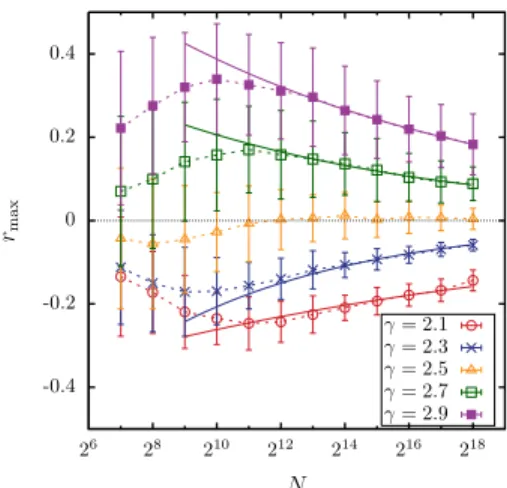
17/4⯝2.56. 共89兲 According to Eq.共88兲,rmaxvanishes for large networks. Note that the value of rmax always remains negative for ␥⬍␥r.

Following the usual definition of assortativity according to the sign of the Pearson coefficient, such networks cannot display assortative mixing at all. For this range of ␥, the dissortative part inKnnis so dominant that it overwhelms the assortative part共see also Fig.5兲. Although some of the esti-mates that lead to Eq. 共88兲 are quite rough, we find good agreement with our simulations, see Fig. 6, where rmax is shown as a function of network sizeNfor different values of

␥. For ␥= 2.1 and ␥= 2.3 the maximal assortativity rmax is indeed found to be negative, ␥= 2.5 shows slightly positive values,␥= 2.7 and ␥= 2.9 clearly positive ones.

V. DISCUSSION

As we have shown above, the correlation profile of scale-free networks exhibits two limiting cases, representing maxi-mally dissortative and assortative mixing. The corresponding

Pearsoncoefficientsrminandrmaxas given by Eqs.共64兲and

-0.4 -0.2 0 0.2 0.4

26 ₂8 ₂10 ₂12 ₂14 ₂16 ₂18

rma

x

N

γ= 2.1 γ= 2.3 γ= 2.5 γ= 2.7 γ= 2.9

FIG. 6. 共Color online兲 Pearsoncoefficientrmaxfor maximally

assortative networks as a function of network sizeN for different values of the scaling exponent␥. All data points are averages over 100 networks with minimal degreek0= 6, error bars denote the

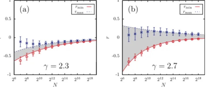
共88兲provide lower and upper bounds for the possible values ofr, as indicated by the shaded area in Fig.7. The region of possiblervalues shrinks with growing network sizeN. In the limit of largeN, bothr_minandr_max vanish, even though the underlying networks are not uncorrelated. Furthermore, it is important to note that networks with ␥ⱕ␥r with ␥r⯝2.5

always exhibit a negative correlation coefficient. As dis-cussed in关18,21兴, this counterintuitive behavior is related to the scaling ofk_maxin Eq.共2兲. The large degree vertices have to export many of their edges into layers of low-degree ver-tices, giving rise to a dissortative part in the network that eventually dominates the overall structure共see also Fig.5兲.

It has been previously recognized that the degree se-quence of networks imposes constraints on their correlation

structure andPearsoncoefficient, see in particular Ref.关28兴, where such constraints have been illustrated for acyclic and small network graphs. In the present study, we addressed the constraints arising from a scale-free degree sequence and ob-tained quantitative results for the structure of maximally cor-related scale-free networks. Furthermore, we have shown in a quantitative manner how this structure evolves as one var-ies the network parametersN,␥, andk0.

We find that these networks are characterized by pro-nounced communities of vertices with the same or similar degree. Dissortative networks exhibit nested bilayers of ver-tices with small degree on the one side and verver-tices with large degree on the other side共see Fig.1兲. Counterintuitively, the number of these bilayers does not grow with network size, but saturates for large networks with given parameters

␥ and k0 关see Eq. 共37兲兴. In Fig. 4 we also find a layered structure for assortative networks, where layers of low-degree vertices withkⱕksform subgraphs, in which all ver-tices have the same degree. The number of these monolayers is limited by large degree vertices, which cannot saturate all their edges by connections to vertices with the same degree. This effect decreases with increasing network size and ks grows monotonously withNas in Eq. 共75兲.

In light of these quantitative results on the layered struc-ture of correlated networks, various structural and dynamical phenomena taking place on them may be better understood, since the analysis can possibly be done separately for each layer.

ACKNOWLEDGMENT

We thank an anonymous referee for making us aware of Refs. 关27,28兴.

关1兴R. Albert and A.-L. Barabási,Rev. Mod. Phys. 74, 47共2002兲.

关2兴M. E. J. Newman,SIAM Rev. 45, 167共2003兲.

关3兴S. N. Dorogovtsev, A. V. Goltsev, and J. F. F. Mendes,Rev. Mod. Phys. 80, 1275共2008兲.

关4兴M. E. J. Newman,Phys. Rev. Lett. 89, 208701共2002兲.

关5兴M. E. J. Newman,Phys. Rev. E 67, 026126共2003兲.

关6兴R. Xulvi-Brunet and I. M. Sokolov,Phys. Rev. E 70, 066102 共2004兲.

关7兴R. Xulvi-Brunet and I. M. Sokolov, Acta Phys. Pol. B 36, 1431共2005兲.

关8兴A. Vázquez and Y. Moreno, Phys. Rev. E 67, 015101共R兲 共2003兲.

关9兴V. M. Eguíluz and K. Klemm, Phys. Rev. Lett. 89, 108701 共2002兲.

关10兴M. Boguñá and R. Pastor-Satorras,Phys. Rev. E 66, 047104 共2002兲.

关11兴M. Boguñá, R. Pastor-Satorras, and A. Vespignani,Phys. Rev. Lett. 90, 028701共2003兲.

关12兴M. Brede and S. Sinha, e-printarXiv:cond-mat/0507710.

关13兴S. J. Wang, A. C. Wu, Z. X. Wu, X. J. Xu, and Y. H. Wang, Phys. Rev. E 75, 046113共2007兲.

关14兴F. Sorrentino, M. Di Bernardo, G. Cuellar, and S. Boccaletti,

Physica D 224, 123共2006兲.

关15兴M. Di Bernardo, F. Garofalo, and F. Sorrentino,Int. J. Bifur-cation Chaos Appl. Sci. Eng. 17, 3499共2007兲.

关16兴R. Cohen, K. Erez, D. Ben-Avraham, and S. Havlin, Phys. Rev. Lett. 85, 4626共2000兲.

关17兴M. Molloy and B. Reed, Random Struct. Algorithms 6, 161

共1995兲.

关18兴M. Boguñá, R. Pastor-Satorras, and A. Vespignani,Eur. Phys. J. B 38, 205共2004兲.

关19兴J. S. Lee, K. I. Goh, B. Kahng, and D. Kim,Eur. Phys. J. B 49, 231共2006兲.

关20兴M. Catanzaro, M. Boguna, and R. Pastor-Satorras,Phys. Rev. E 71, 027103共2005兲.

关21兴S. Weber and M. Porto,Phys. Rev. E 76, 046111共2007兲.

关22兴S. Maslov and K. Sneppen,Science 296, 910共2002兲.

关23兴S. Maslov, K. Sneppen, and A. Zaliznyak,Physica A 333, 529 共2004兲.

关24兴R. Pastor-Satorras, A. Vázquez, and A. Vespignani,Phys. Rev. Lett. 87, 258701共2001兲.

关25兴A. Vazquez, R. P. Satorras, and A. Vespignani, Phys. Rev. E 65, 066130共2002兲.

关26兴M. Boguñá and R. Pastor-Satorras,Phys. Rev. E 68, 036112 -1

-0.5 0 0.5 1

26 28 210 212 214 216 218

r

N rmin

rmax (a)

-1 -0.5 0 0.5 1

26 28 210 212 214 216 218

r

N rmin

rmax (b)

γ= 2.3 γ= 2.7

FIG. 7. 共Color online兲 Pearson coefficients rmin and rmax for

maximally correlated networks as a function of network sizeNfor networks with k0= 6 and scaling exponent 共a兲 ␥= 2.3 and 共b兲 ␥

= 2.7. Data points and fits from relations共64兲and共88兲are identical to the corresponding curves in Figs. 3 and 6. The shaded areas indicate the range of possiblervalues for any realization of a scale-free network with the corresponding parameters共N,␥,k0兲. For

net-works with␥= 2.3 as in panel共a兲, allrvalues are negative. In both

共2003兲.

关27兴M. A. Serrano, M. Boguñá, R. Pastor-Satorras, and A. Vespig-nani, inLarge Scale Structure and Dynamics of Complex Net-works: From Information Technology to Finance and Natural Science, edited by G. Caldarelli and A. Vespignani共World Sci-entific, Singapore, 2007兲, pp. 35–66.

关28兴D. L. Alderson and L. Li,Phys. Rev. E 75, 046102共2007兲.

关29兴For assortative networks, this restriction is essential in order to avoid the trivial case of maximal assortativity, where all verti-ces are connected only to themselves. In the dissortative case,

multiple connections do not play an important role, since the hubs can saturate all their connections with different low-degree vertices.

关30兴Sometimes the so-called excess degreekex⬅k− 1 is considered

instead, which leads to some mathematical simplifications.