Asymptotic Inference for Dynamic Panel Estimators of Infinite
Order Autoregressive Processes
∗Yoon-Jin Lee†, Ryo Okui‡ and Mototsugu Shintani§
This version: November 2016
Abstract
In this paper we consider the estimation of a dynamic panel autoregressive (AR) process
of possibly infinite order in the presence of individual effects. We employ double asymptotics
under which both the cross-sectional sample size and the length of time series tend to infinity
and utilize the sieve AR approximation with its lag order increasing with the sample size. We
establish the consistency and asymptotic normality of the fixed effects estimator and propose a
bias-corrected fixed effects estimator based on a theoretical asymptotic bias term. Monte Carlo
simulations demonstrate the usefulness of bias correction. As an illustration, the proposed
methods are applied to dynamic panel estimation of the law of one price deviations among US
cities.
Key Words: autoregressive sieve estimation; bias correction; double asymptotics; fixed effects estimator.
JEL Classification: C13; C23; C26.
∗The authors thank Oliver Linton (the editor), associate editor, two anonymous referees, Kazuhiko Hayakawa, Igor
Kheifets, Simon Lee, Yoonseok Lee, Yoshihiko Nishiyama, Tatsushi Oka, Laurent Pauwels, Peter Phillips, Yoon-Jae Whang, and seminar and conference participants at the Asian Meeting of the Econometric Society in Delhi, Erasmus School of Economics, the 20th International Panel Data Conference, the Kansai Econometric Society Meetings in Osaka, Kyoto University, the 2011 Meetings of the Midwest Econometrics Group in Chicago, North Carolina State University, Nanyang Technological University, the National University of Singapore, 2014 North American Summer Meeting of the Econometric Society at Minnesota University, Otaru University of Commerce, SETA2012, SKK International Workshop in Kyoto, Singapore Management University, and 2015 Workshop on Advanced Econometrics at Kansas University for their helpful comments and discussion. Haruo Iwakura provided excellent research assistance. Okui appreciates financial support from the Japan Society of the Promotion of Science under KAKENHI 22730176, 22330067, 25285067, 25780151, 15H03329 and 16K03598. Shintani gratefully acknowledges financial support by the National Science Foundation Grant SES-1030164 and KAKENHI26285049.
†Department of Economics, Kansas State University, Manhattan, KS 66501, USA. Email: yoonjin@ksu.edu ‡Institute of Economic Research, Kyoto University, Yoshida-Hommachi, Sakyo, Kyoto, Kyoto, 606-8501, Japan,
and Department of Economics, University of Gothenburg, P.O. Box 640, SE-405 30 Gothenburg, Sweden. Email: okui.ryo.3@gmail.com
§RCAST, the University of Tokyo, Meguro-ku, Tokyo 153-8904, Japan, and Department of Economics, Vanderbilt
1
Introduction
In recent decades, an increasing number of panel data sets with longer time series have become
available for economic analysis. In this paper, we investigate the possible benefits of using such panel
data in estimating a general dynamic structure described by an infinite order panel autoregressive
(AR) model. To this end, we follow recent studies in dynamic panel analyses by using an asymptotic
approximation with not only a cross-sectional dimensionN but also a time series dimensionT that
tends to infinity. For example, using this type of asymptotic framework, Hahn and Kuersteiner
(2002), Alvarez and Arellano (2003) and Hayakawa (2009) among others, have investigated the
properties of various estimators for finite order panel AR models. We consider a more general
dynamic linear model that is less subject to problems caused by possible model misspecification.1
Our approach is to approximate a panel AR model of infinite order by letting the AR order p
increase withT. Such an idea of the AR sieve approximation in estimating a general linear model
has long been used in the time series analysis literature. To the best of our knowledge, however,
it has yet to be used in the inference of dynamic panel models. It is our intention to fill the gap
between these two bodies of literature.
There are a number of important empirical issues to which our method can be applied. In
macroeconomic analysis, the long-run cumulative effect of productivity or demand shocks on the
economy is often of interest and time series data have been used to measure the persistence of
shocks. Once the general linear model is expressed as an AR model of infinite order, the sum of the
AR coefficients (SAR) can be used as a formal measure of the persistence. The AR sieve estimator
of the SAR, however, is known to converge at a rate of pT /p which is slower than the order of
√
T. By incorporating cross-sectional information, our dynamic panel procedure can offer increased
1
precision of the persistence estimator with its convergence rate pN T /p which can be faster than
√
T. As an empirical illustration, we estimate the SAR of the law of one price (LOP) deviations
among US cities based on the micro price panel data of individual goods used in Crucini, Shintani
and Tsuruga (2015). Another useful application of our approach is the literature on dynamic panel
vector AR (VAR) models. Allowing for heterogeneity among households and firms by using micro
data has become an important issue in recent VAR analyses. For example, Franco and Philippon
(2007) and Head, Lloyd-Ellis and Sun (2014), among others, estimate structural panel VAR models
with a moderately large number of time series observationsT. The use of such VAR models without
prespecifying the lag length can be justified by our results for the multivariate case.
We begin our analysis with the fixed effects (FE) estimator. Under some regularity conditions,
we show the consistency and asymptotic normality of the FE estimator which are comparable to
those of the ordinary least squares (OLS) estimator in a time series setting, including the ones
obtained by Lewis and Reinsel (1985). The presence of the individual fixed effects in the dynamic
panel setting, however, makes the analysis more complicated than in the time series setting, creating
an asymptotic bias of order √p/T. If an intercept term is included in the analysis of Lewis and
Reinsel (1985), there will also be a bias term of the same order. However, it converges to zero
at a rate faster than the rate of convergence of the OLS estimator (√T) because √T ×√p/T =
p
p/T →0 underp/T →0 which is implied by the rate conditions used to prove the consistency and
asymptotic normality of the OLS estimator. Therefore, no bias term shows up in the asymptotic
distribution whenN = 1. In panel data settings, the order of the bias of the FE estimator is still
√p/T, but the FE estimator converges at a faster rate of√N T. As a consequence, the asymptotic
distribution is contaminated by a bias of order ppN/T (=√N T ×√p/T).
Because of the incidental parameters problem of Neyman and Scott (1948), the FE estimator
in dynamic panel data models is known to be biased whenN/T is not very small (see, e.g., Nickell,
paper is that the bias can be even more problematic in the estimation of panel AR models of
infinite order because the bias increases with the lag orderp used in the AR sieve approximation,
so that using a sieve AR approach to mitigate the effects of lag order misspecification can adversely
contribute to a larger bias.
To eliminate the increased magnitude of the first order bias, we propose a bias-corrected FE
(BCFE) estimator based on the consistent estimator of the theoretical bias term. A Monte Carlo
simulation suggests that our proposed BCFE estimator works well in reducing the bias of the FE
estimator which is not negligible with the sample sizes typically available in practice.2 Based on
the theoretical results for the asymptotic normality, we can consider asymptotically valid standard
errors and an asymptotically valid automatic lag selection procedure in an AR sieve approximation,
both of which are useful in conducting inference.
The remainder of this paper is organized as follows. Our model is described in Section 2.
The FE estimator and the BCFE estimators are introduced and their asymptotic properties are
investigated in Section 3. The finite-sample performance of the estimators is examined in Section 4,
and our approach is applied to the real data in Section 5. Concluding remarks are made in Section
6. All mathematical proofs are collected in the appendix and the supplemental material available
on the authors’ web sites.
We use the following notation: for a sequence of vectorait, we letat= (a1t, . . . , aN t)′. The same
convention applies to a sequence of a vector denoted by ait(p) so that at(p) = (a1t(p), . . . , aN t(p))′.
A constant C represents an arbitrary constant.
2
The Model
Suppose that we observe panel data {{yit}Tt=1}Ni=1. We assume that yit is generated from an
2
AR process of possibly infinite order with individual specific effects. Namely, the model is:
yit=µi+ ∞ X
k=1
αkyi,t−k+ǫit, (1)
whereµi is an unobservable individual effect and ǫit is an unobservable innovation with mean zero
and variance σ2. The AR parameters, {αk}∞k=1, are assumed to be identical acrossi: namely, we
assume that the dynamics are homogeneous across observational units. The individual effect, µi,
is included in order to capture the heterogeneity across individuals. Controlling for unobserved
heterogeneity using individual effects is an important advantage of panel data analysis. The
sta-tionarity of yit is imposed throughout the paper. In what follows, we consider the situation in
which both the cross-sectional sample size,N, and the length of the time series, T, are large.
The specification (1) is quite general and can include various linear stationary time series such
as stationary and invertible panel autoregressive-moving-average (ARMA) models with individual
effects. Much applied work, especially in time series, relies on this representation.
To estimate (1), we follow the time series literature on AR sieve estimation and utilize its
approximated model:
yit=µi+ p X
k=1
αkyi,t−k+uit,p, (2)
whereuit,p=bit,p+ǫit withbit,p=P∞k=p+1αkyi,t−k. The term bit,p represents the error caused by
approximating the true infinite order AR model given by (1) using the AR model with a truncated
lag,p, given by (2). This approximated model is convenient in maintaining the computational
sim-plicity of the parametric finite order AR model while making the effect of the model misspecification
disappear asymptotically.
We make the following assumptions throughout the paper.
Assumption 1. (i) {ǫit} is independently and identically distributed (i.i.d.) over time and across
individuals with mean zero, 0 < E(ǫ2it) = σ2 < ∞, and E|ǫit|2r ≤ C, for some r > 2; (ii) ǫit is
yi,1−s, s= 0,1,2, . . ., are generated from the stationary distribution; (v) p1/2P∞k=p+1|αk| →0 as
p→ ∞.
We note that Lewis and Reinsel (1985) impose assumptions similar to Assumption 1 to estimate
the AR estimators in time series.3 In Assumption 1(i), we focus on i.i.d. errors {ǫ
it} for the sake
of simplicity, as in Lewis and Reinsel (1985). The i.i.d. error assumption can be relaxed to allow
for a martingale difference sequence at the cost of stronger moment conditions, as in Gon¸calves
and Killian (2007). Assumption 1(ii) is used for the moving average representation of the model.
Assumption 1(iii) indicates thatyitis stationary and can be represented by an infinite order moving
average process. Considering cases in whichyit is an integrated process is beyond the scope of this
paper. Assumption 1(iv) can be relaxed because the influence of the initial observations is not
decisive when T is sufficiently large. However, relaxing it would make the mathematical argument
extremely tedious. Assumption 1(v) is a commonly used assumption in the literature on AR sieve
estimation, which implies that the approximation error should not be too large. This assumption
imposes smoothness on the spectral density of the process.
It is also useful for our purpose to introduce an infinite order moving average representation of
(1):
yit=ηi+ ∞ X
k=0
ψkǫi,t−k,
where ψ0 ≡ 1, P∞j=0|ψj| < ∞ and ηi = µi/(1−P∞k=1αk). This representation is justified by
Assumption 1.
Let Γpbe the variance–covariance matrix of the vector (wit, . . . , wi,t−p+1)′wherewit=yit−ηi= P∞
k=0ψkǫi,t−k. Note that Γp does not depend oni. Assumption 1 implies that Γp is positive definite
and its eigenvalues do not diverge.
3
3
Main Results
This section introduces the conventional FE estimator to estimate parameters in the
approxi-mated model (2). We then show the asymptotic property of the estimator and compare it to that
used in time series estimation, namely that of Lewis and Reinsel (1985). A BCFE estimator is also
developed.
3.1 The FE estimator
To define the estimator, we introduce the vector representation of the approximated model (2)
as follows:
yit=µi+xit(p)′α(p) +uit,p (3)
where xit(p) = (yi,t−1, . . . , yi,t−p)′ and α(p) = (α1, . . . , αp)′. The first step in FE estimation is to
eliminate the individual effects by subtracting individual averages. Let
˜
yit = yit−
1
T−p(yi,p+1+· · ·+yiT),
˜
xit(p) = xit(p)−
1
T−p(xi,p+1(p) +· · ·+xiT(p))
and ˜uit,p be similarly defined. By rewriting the model (3) in terms of the transformed variables,
we have:
˜
yit= ˜xit(p)′α(p) + ˜uit,p, (4)
which does not contain the individual effects. Applying OLS to (4) yields the FE estimator, denoted
by ˆαF(p):
ˆ
αF(p) =
T X
t=p+1
˜
xt(p)′x˜t(p)
−1
T X
t=p+1
˜
xt(p)′y˜t.
We define consistency as the property that the probability limit of the distance between the
estimator and the true value of the parameter converges to zero where we use the Euclidean distance
||a||=√a′afor a vector a.4 The following theorem shows the consistency of ˆα F(p).
4
Theorem 1. Suppose that Assumption 1 is satisfied. Then, if N → ∞, T → ∞ andp → ∞with
p2/(Tmin(N, T))→0, we have:
||αˆF(p)−α(p)|| →p 0.
Next we show the asymptotic normality of a linear combination of the estimated AR parameters.
Let ℓp be an arbitrary deterministic sequence of p×1 vectors such that 0< C1 ≤ ||ℓp||2 =ℓ′pℓp ≤
C2 < ∞ for p = 1,2,· · · for some C1 and C2.5 Our parameter of interest is limp→∞ℓ′pα(p). For
example, if we are interested in the kth AR coefficient, αk, for 1 ≤k ≤p, our choice of ℓp would
be ek = (0, . . . ,0,1,0, . . . ,0)′ where ek is a p×1 selection vector with the kth element being one
and other elements being zero.
The following theorem presents the asymptotic distribution of the FE estimator ℓ′
pαˆF(p). Let
v2
p = σ2ℓ′pΓ−1p ℓp, which turns out to be the asymptotic variance of all the estimators considered
in this paper. Note that Assumption 1(iii) guarantees that the maximum eigenvalue of Γ−1p is
bounded, which implies thatvp2 is bounded away from zero.
Theorem 2. Suppose that Assumption 1 is satisfied. Then, if N → ∞, T → ∞ andp → ∞with
√
N TP∞k=p+1|αk| →0, p2/T →0 and p3N/(Tmin(N2, T2))→0, we have:
p
N(T −p)ℓ′pαˆF(p)−ℓ′pα(p) +ℓ′pΓ−1p B/T
/vp→dN(0,1),
where
B = 1 (T −p)
T X
t=p+1 t−1 X
m=p+1
σ2ψt−−1−m(p),
wik(p) = (wi,k, . . . , wi,k−p+1)′and ψt−−1−m(p) = (ψt−1−m, ψt−2−m, . . . , ψt−p−m).
The theorem shows that ℓ′
pαˆF(p) is asymptotically normal, but also asymptotically biased. We
see as well that the convergence rate ofℓ′
pαˆF(p) is
√
N T when we ignore the bias term. The result
that our definition of consistency is actually stronger than this alternative definition. This is because supk|αˆk−αk| ≤
||αˆ(p)−α(p)||+ supk>p|αk| →p0 if||αˆ(p)−α(p)|| →p0 andp→ ∞.
5
in Theorem 2 extends that in Theorem 4 of Lewis and Reinsel (1985) from the time series context
to the panel data context.
A caveat is that the above result does not immediately imply thatpN(T −p)[ℓ′
pαˆF(p)−ℓ′pα(p)+
ℓ′
pΓ−1p B/T]→dN(0,limN,T→∞vp2). Additional conditions would be required for the convergence of vp and the weak convergence of pN(T−p)ℓ′pαFˆ (p)−ℓ′pα(p) +ℓ′pΓ−1p B/T. Note that the same
comment applies to the results of Lewis and Reinsel (1985). See Kuersteiner (2005) for this point.
Nonetheless, we show in the above theorem that once divided byvp, p
N(T−p)[ℓ′
pαˆF(p)−ℓ′pα(p)+
ℓ′
pΓ−1p B/T]/vp, weakly converges to the standard normal distribution and we note that this result
is useful for inference.
3.2 Comparisons with the OLS estimator in univariate time series
In this section, we carefully compare our asymptotic results of the FE estimator for an infinite
order panel AR model with those of the univariate version of Lewis and Reinsel (1985). If we set
N = 1, our model reduces to a conventional infinite order AR process of which the estimators
and their asymptotic theory have long been developed in the literature on time series analysis,
including Berk (1974), Lewis and Reinsel (1985), L¨utkepohl and Poskitt (1991), L¨utkepohl and
Saikkonen (1997) and Gon¸calves and Kilian (2007), among others. However, applying this sieve
AR framework is new in dynamic panel data analysis.
First, the result in Theorem 1 can be viewed as an extension of the consistency of AR coefficient
estimators from a time series to a panel data context. The main difference between this result and
that of Lewis and Reinsel (1985) is that the required condition in our case isp2/(Tmin(N, T))→0
but in the case of time series it is p2/T → 0. To understand the role of our condition, it is useful
to note that p2/(Tmin(N, T)) → 0 is equivalent to p2/(N T) → 0 and p/T → 0. The first part
p2/(N T)→ 0 is the condition for the variance to tend to 0, as a large N reduces the variance in
a panel data setting. Note that p2/T → 0 is the corresponding condition for Lewis and Reinsel
Second, the result in Theorem 2 extends that in Theorem 4 of Lewis and Reinsel (1985) from
the time series context to the panel data context. However, unlike in time series, ℓ′
pαˆF(p) is
asymptotically biased. This asymptotic bias is what distinguishes our analysis from that of time
series.
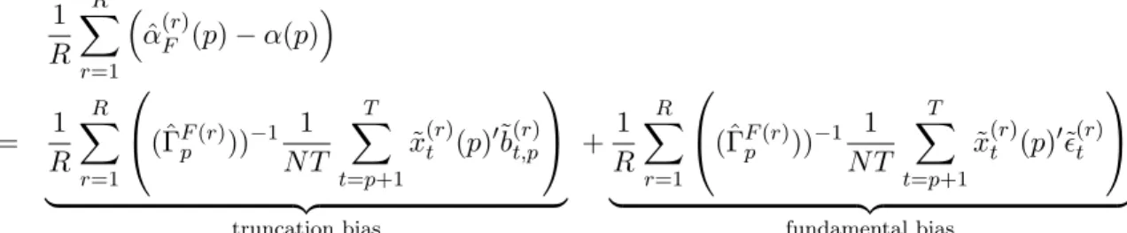
To better understand the structure of the bias in our analysis, we can utilize a convenient
decomposition formula. As uit,p = bit,p +ǫit, the transformed error ˜uit,p is the sum of ˜bit,p =
bit,p−PTt′=p+1bit′,p/(T−p) and ˜ǫit=ǫit−PTt′=p+1ǫit′/(T−p). For this reason, the total bias can
be decomposed as:
E(ˆαF(p)−α(p))
= E
(ˆΓFp)−1 1 N(T−p)
T X
t=p+1
˜
xt(p)′u˜t,p
= E
(ˆΓFp)−1 1 N(T−p)
T X
t=p+1
˜
xt(p)′˜bt,p
| {z }
truncation bias
+E
(ˆΓFp)−1 1 N(T−p)
T X
t=p+1
˜
xt(p)′˜ǫt
| {z }
fundamental bias
,
where
ˆ
ΓFp = 1
N(T −p)
T X
t=p+1
˜
xt(p)′x˜t(p).
The first term is the bias that arises because we estimate the AR model with a truncated
lag length, not the true infinite order AR model. Throughout the paper, we refer to this bias as
‘truncation bias.’ Similarly, we refer to the second term as ‘fundamental bias’ because this part of
the bias is present even if we estimate the true finite order AR model with the correct lag length.
While the truncation bias may not be negligible in finite samples, it vanishes in our asymptotic
analysis because of our assumption√N T P∞k=p+1|αk| →0. This assumption implies thatp, N and
T should satisfy supk>p+1|αk|=o(√N T). Ifpincreases very slowly, the approximation error does
not vanish fast enough and a bias of the estimator appears. For example, if wit follows a finite
order stationary and invertible ARMA process,αk decays exponentially andpmust grow at a rate
It is the second term, namely the fundamental bias, that appears in Theorem 2. We impose
the condition, √N T P∞p+1|αk| → 0, in the theorem so that the truncation bias vanishes. The
reason that we impose this condition to only present the fundamental bias in the theorem is that
the truncated bias cannot be estimated whereas the fundamental bias can be estimated and a
bias-corrected estimator can be developed. The order of the fundamental bias term is √p/T, which
is the same order as that in a general time series model. However, it may affect the asymptotic
distribution because √N T ×√p/T may not converge to 0.
To gain further insight into the bias, we will make a parallel comparison with a time series
analysis. Consider a truncated representation of a univariate AR model of infinite order.
yt=µ+xt(p)′α(p) +ut,p
whereut,p =bt,p+ǫtwithbt,p =P∞k=p+1αkyt−k,xt(p) = (yt−1, . . . , yt−p)′ and α(p) = (α1, . . . , αp)′.
Consider an OLS estimator ˆαOLS(p):
ˆ
αOLS(p) =
T X
t=p+1
˜
xt(p)˜xt(p)′
−1
T X
t=p+1
˜
xt(p)˜yt,
where ˜xt(p) =xt(p)−PTt′=p+1xt′(p)
/(T−p) and ˜yt(p) =yt(p)−PTt′=p+1yt′(p)
/(T−p). We
can consider a similar bias decomposition as in the panel data case
E(ˆαOLS(p)−α(p))
= E
(ˆΓp)−1
1
T−p T X
t=p+1
˜
xt(p)˜bt,p
+E
(ˆΓp)−1
1
T −p T X
t=p+1
˜
xt(p)˜ǫt
where
ˆ
Γp= 1 T −p
T X
t=p+1
˜
xt(p)˜xt(p)′,
˜bt,p = bt,p −PT
t′=p+1bt′,p/(T −p), and ˜ǫt = ǫt−PT
t′=p+1ǫt′/(T −p). The second term above is
the fundamental bias6 as in the panel data case and is of order√p/T.7 However, the fundamental
6
We note that the fundamental bias term here is essentially identical to the term that causes incidental parameter bias in the panel AR(1) model.
7
bias does not affect the asymptotic distribution of ˆαOLS(p) in time series settings. The asymptotic
bias vanishes because √T(√p/T) =pp/T →0 given the convergence rate of ˆαOLS(p) at
√
T and
the lag growth condition of p/T → 0, which is implied by the rate conditions for the consistency
and asymptotic normality of ˆαOLS(p). On the other hand, in general, the asymptotic bias may
remain in the panel data setting because √N T(√p/T) =ppN/T may not converge to zero given
ˆ
αF(p) converges at a rate√N T. Even ifp/T →0 is satisfied,N can be of the same or larger order
than (p/T)−1. In the special case of fixed and finite p, the asymptotic bias becomes proportional
to the limit of pN/T. This case corresponds to the well-known outcome that the FE estimator is
asymptotically biased in dynamic panel data models with finite AR lags (see, e.g., Nickell, 1981,
Kiviet, 1995, Hahn and Kuersteiner, 2002 and Lee, 2012). In the context of increasingp,N/T →0
is not sufficient for the bias to vanish and the bias is increasing with p. Therefore, we note that
using the sieve AR approach to mitigate the effects of lag order misspecification can adversely
contribute to a larger incidental parameter bias.
3.3 BCFE estimator
We now consider a bias correction. We correct the bias by using ˆB/T = (ˆσ2/(1−Ppk=1α˜k))ιp/(T−
p), where ιp is the p ×1 vector of ones and ˜αk are the FE estimators for αk. We note that
B/T ≈σ2P∞k=0ψkιp/(T−p) andP∞k=0ψk = 1/(1−P∞k=1αk). Thus, ˆB may be a natural
estima-tor ofB. Our BCFE estimator is given by:
ˆ
αBF(p) = ˆαF(p) + (ˆΓFp)−1B/T.ˆ
The following theorem gives the consistency of the BCFE estimator.
Theorem 3. Suppose that Assumption 1 is satisfied. Then, if N → ∞, T → ∞ andp → ∞with
p2/(Tmin(N, T))→0, we have:
||αˆBF(p)−α(p)|| →p 0.
Theorem 4. Suppose that Assumption 1 is satisfied. Then, if N → ∞, T → ∞ and p → ∞
with √N T P∞k=p+1|αk| →0, p3/(Tmin(N, T))→0,p2/T →0 and p3N/(Tmin(N2, T2))→0, we
have:
p
N(T−p)ℓ′p( ˆαBF(p)−α(p))
/vp →dN(0,1).
This theorem shows that our bias-corrected estimator can effectively eliminate the asymptotic
bias. It is remarkable that this bias correction does not inflate the bias asymptotically.
3.4 Estimation of the sum of the AR coefficients
The sum of the AR coefficients (SAR) defined by
SAR=
∞ X
k=1 αk,
can capture the long-run cumulative effect of a shock. We pay special attention to this measure
because of its importance in empirical applications. The SAR can be estimated as:
[
SARF =√pℓ∗′pαˆF(p)
withℓ∗
p =ιp/√p= (1/√p, . . . ,1/√p)′ whereιp is ap×1 vector of ones.
Based on the results of Theorem 2, we have two remarks regarding the estimation of SAR.
First, from the results in Theorem 2, the convergence rate of SAR[F is p
N T /p, which is slower
than √N T. Second, the asymptotic distribution of SAR[F can be presented around SAR. Note
that the difference betweenSARandPpk=1αkisP∞k=p+1αkwhich is of smaller order than p
N T /p
by the assumption√N TP∞k=p+1|αk| →0. This observation implies that the asymptotic results in
Theorem 2 hold even if we replace ℓ′
pα(p) withSAR/√p. The same remark applies to the BCFE
estimator.
For SAR[F, a simple bias-correction method can be employed. In this case, we haveℓ∗′pΓ−1p ιp≈
√p(1−P∞
by solving:
1
√pSAR[BF =
1
√pSAR[F +
√p
T−p(1−SAR[BF),
so that
[
SARBF = T−p
T SAR[F + p
T. (5)
This BCFE estimator may be considered the limit of iterating the bias correction (see, e.g., Hahn
and Newey (2004, p. 1299)).8
3.5 Standard errors
Computing the standard errors of the FE and BCFE estimators requires the consistent
estima-tion ofv2
p =σ2ℓ′pΓ−1p ℓp. A natural estimator ofvp2 is:
ˆ
v2p,F =
1
N(T −p)
N X
i=1 T X
t=p+1
(˜yit−x˜it(p)′αˆF(p))2
ℓ′p(ˆΓFp)−1ℓp.
Alternatively, one may estimate vp2 by using ˆαBF(p) in place of ˆαF(p). We denote this variance
estimator by ˆvp,BF.
The following theorem shows the consistency of the variance estimators ˆvp,F2 and ˆvp,BF2 .
Theorem 5. Suppose that Assumption 1 is satisfied. If N → ∞, T → ∞ and p → ∞ with
p2/(Tmin(N, T))→0, then ˆv2p,F −vp2→p0 and vˆp,BF2 −v2p →p 0.
The proof is in the supplemental material.
The variance estimators are consistent when ˆαF(p) and ˆαBF(p) are consistent. Note that
additional assumptions are required to show that vp converges and this is the reason why we state
the result as ˆvp,F2 −v2p →p 0 but not ˆvp,F2 →p vp. Nonetheless, this result is sufficient for our purpose.
8
3.6 Lag selection
The estimation procedures require the lag order of the approximated model, p, to be chosen
by researchers. In choosing p, we consider the following general-to-specific rule. This automatic
rule follows a procedure similar to the one considered in Ng and Perron (1995) which tests for the
significance of the coefficients on lags.9
Each step of the general-to-specific rules uses the t-statistic for the coefficient on the highest
lag in the model. Let ep be the p×1 vector whose pth element is 1 and other elements are zero.
Let
tp(ˆα(p)) =
√
N T e′pαˆ(p)/vˆp,
where ˆα(p) and ˆvp are estimators of α(p) andvp withℓp =ep, respectively. The statisticstp(ˆα(p))
are thet-test statistics for the null hypothesis αp = 0 based on estimator ˆα(p).
The general-to-specific procedure is the following. We a priori set the maximum possible value
ofp, denotedpmax. Let ˆpbe the maximum value ofpsuch that|tp(ˆα(p))|> z0.5α, wherez0.5α is the
upper 0.5α quantile of the standard normal distribution, for p = 1,2, . . . , pmax. This ˆp is the lag
length chosen by this general-to-specific procedure. An alternative explanation of the rule is the
following. We keep thepth-lag if its coefficient is statistically significant in the AR(p) specification.
Otherwise, we drop the pth-lag, estimate the AR(p−1) model and test the significance of the
coefficient of the (p−1)th-lag. We repeat this process until the coefficient becomes statistically
significant or p reaches zero.
The following theorem gives the rate of ˆp.
Theorem 6. Suppose that Assumption 1 is satisfied. Let pmin be such that pmin < pmax, pmax−
9
pmin → ∞, and √N T pmaxP∞k=pmin+1|αk| → 0 as N, T, pmin, pmax → ∞. Suppose that N, T and
p =pmax satisfy the conditions p
N(T−p)ℓ′
p(ˆα(p)−α(p))/vp →dN(0,1) and vˆp →p vp. Then it
holds that P(ˆp < pmin)→0 asN, T, pmin, pmax→ ∞.
The proof is in the supplemental material.
This theorem implies that we can choose p using the general-to-specific procedure such that
it satisfies the requirement for the asymptotic normality of an estimator by appropriately setting
the rate of pmax. In the simulations presented below, we set pmax =O(T1/4) under which all the
conditions for the theoretical analysis hold.
3.7 Multivariate extension
Although we focus on a univariate panel data model, the results of the paper can be extended
to multivariate panel data models. In this section, we outline the multivariate generalizations of
the estimation of the univariate panel model developed in the previous sections to highlight the
potential wide applicability of our methodology.
Consider a multivariate panel AR model of infinite order:
Yit=µi+
∞ X
k=1
AkYi,t−k+Eit,
whereYit is an r×1 vector, Ak is anr×r matrix of coefficients,µi is an r×1 vector of individual
effects, and Eit is anr×1 vector of unobservable innovations which is a sequence of i.i.d. random
vectors with mean 0 and positive definite covariance matrix Σ. Similarly to the univariate case, we
can approximate the model by:
Yit=µi+
p X
k=1
AkYi,t−k+Uit,
where Uit = P∞k=p+1AkYi,t−k +Eit. Let Xit(p) = (Yi,t′ −1, . . . , Yi,t′ −p)′ (an rp×1 vector) and
matrix notation as:
Yit=µi+A(p)Xit(p) +Uit.
To define the FE estimator, we first eliminate the fixed effects via a transformation. Let ˜Yit=
Yit−PTs=p+1Yis/(T−p), ˜Xit(p) =Xit(p)−PTs=p+1Xis(p)/(T−p), and ˜Uit=Uit−PTs=p+1Uis/(T−
p). Then, the transformed variables satisfy:
˜
Yit=A(p) ˜Xit(p) + ˜Uit. (6)
Let ˜Yt= ( ˜Y1t, . . . ,YN t˜ )′, an N ×r matrix. Similarly, let ˜Xt(p) = ( ˜X1t(p), . . . ,XN t˜ (p))′, an N×rp
matrix, and Et = (E1t, . . . , EN t)′, an N ×rp matrix. Applying OLS to (6), we obtain the FE
estimator for the multivariate panel data model as follows:
ˆ
AF(p) =
T X
t=p+1
˜
Yt′Xt˜ (p)
T X
t=p+1
˜
Xt(p)′Xt˜ (p)
−1
.
Let ℓpr be an arbitrary deterministic sequence of pr×1 vectors such that 0 < C1 ≤ kℓprk2 ≤
C2<∞forp= 1,2, . . . for someC1 and C2. Let
Vp2=ℓ′pr Γ−1p ⊗Σℓpr,
whereΓpis anrp×rpmatrix whose (m, n)th (r×r) block of elements isE((Yit−µi)(Yi,t+m−n−µi)′).
We also impose the following assumption.
Assumption 2. (i) {Eit}is independently and identically distributed (i.i.d.) over time and across
individuals with mean zero, 0 < E(EitEit′) = Σ < ∞, and E|eit,k|2r ≤ C for any k and some
r > 2, where eit,k is the k-th element of Eit; (ii) Eit is independent of µi for all i and t; (iii)
P∞
k=0kAkk<∞ anddet(P∞k=0Akzk)= 06 for any|z| ≤1; (iv) Yi,1−s,s= 0,1,2, . . ., are generated
from the stationary distribution; (v) p1/2P∞k=p+1kAkk →0 asp→ ∞.
This assumption is a multivariate analog of Assumption 1. In Theorem 7, we derive the
Theorem 7. Suppose that Assumption 2 is satisfied. If N → ∞, T → ∞ and p → ∞ with
p2/(Tmin(N, T))→0, then we have:
kAˆF(p)−A(p)k →p 0.
IfN → ∞,T → ∞andp→ ∞with√N T P∞k=p+1kAkk →0,p2/T →0andp3N/(Tmin(N2, T2))→
0, then:
p
N(T −p)ℓ′prvec
ˆ
AF(p)−A(p) +
B
TΓ −1 p
/Vp→dN(0,1),
where
B= T (T −p)2
T X
t=p+2 t−1 X
m=p+1
ΣΨt−1−m(p),
Ψk(p) = (Ψ′k, . . . ,Ψ′k−p+1) andΨk is the k-th order coefficient matrix of an MA(∞) representation
of Yit.
The proof is in the supplemental material and is similar to those of Theorems 1 and 2.
We also consider a bias-corrected estimator. Let
ˆ
Γp =
1
N(T −p)
T X
t=p+1
˜
Xt(p)′X˜t(p),
and
ˆ
B= T
T−pΣˆ Ir− p X
k=1
ˆ
A′k !−1
⊗ιp,
where ˆAks are the FE estimators and Ir is the r×r identity matrix. Our BCFE estimator for
multivariate models is given by:
ˆ
ABF(p) = ˆAF(p) + ˆBΓˆ −1 p /T.
Theorem 8. Suppose that Assumption 2 is satisfied. If N → ∞, T → ∞ and p → ∞ with
p2/(Tmin(N, T))→0, then we have:
kAˆBF(p)−A(p)k →p 0.
If N → ∞, T → ∞ and p→ ∞ with √N T P∞k=p+1kAkk →0, p3/(Tmin(N, T))→ 0, p2/T → 0
and p3N/(Tmin(N2, T2))→0, then
p
N(T −p)ℓ′prvecAˆBF(p)−A(p)
/Vp →dN(0,1).
The proof is in the supplemental material and is similar to those of Theorems 3 and 4.
4
Monte Carlo Experiments
In this section, we conduct Monte Carlo simulations to evaluate the accuracy of our asymptotic
results on various dynamic panel estimators in finite samples. We generate samples from the
following ARMA(1,1) model:
yit=ηi+φyi,t−1+ǫit+θǫi,t−1,
whereφ={0.5,0.99},θ= 0.4 andηi∼N(0,1) is independent acrossi,ǫit∼N(0,1) is independent
acrossiandt. The individual effectηiand idiosyncratic errorǫitare also independently drawn. We
estimate the first AR coefficient α1 and the sum of the AR coefficients (SAR) P∞k=1αk using the
FE estimator ˆαF(p) and the BCFE estimator ˆαBF(p). Whenφ= 0.5 (DGP1), trueα1 and SAR are
0.9 and 0.643, respectively. Whenφ= 0.99 (DGP2), the impulse response function is hump-shaped
with true α1 being 1.390 and the process becomes highly persistent with the true SAR being near
unity at 0.993. For each process, yi0 are generated from the (conditional) stationary distribution:
yi0|ηi ∼N
ηi
1−φ,
1 +θ2+ 2φθ
1−φ2
.
The pairs of N and T we consider are taken from the set {25,50,100}. All the Monte Carlo
For the choice of lag length pin approximated AR models, we consider both the fixed case and
automatically selected case. For the fixed case, we follow a conventional rule of thumb from the
time series literature and use p= [12(T /100)1/4] where [x] is the integer part ofx. This fixed rule
provides p = 8, 10 and 12 for T = 25, 50 and 100, respectively. The automatic lag selection rule
corresponds to the general-to-specific procedure described in Section 3.6 with the maximum lag set
at pmax = [12(T /100)1/4] and the significance level set at α = 0.1.10 This implies the automatic
procedure always selects lag lengths shorter than or equal to the ones using the fixed rule. At the
same time, it should be noted that both the fixed case and automatically selected case satisfy the
required conditions in the theoretical analysis.
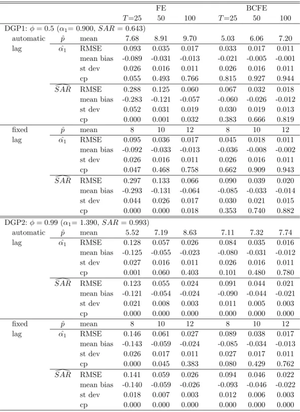
Table 1 shows the root mean squared error (RMSE), mean bias, standard deviation (st dev) and
coverage probability of an asymptotic 95% confidence interval whenN = 100 andT ={25,50,100}.
It also presents the mean values of lag length chosen by the automatic lag selection rule.
The results clearly illustrate the bias properties of the estimators and are consistent with the
theoretical predictions. The FE estimator suffers from the bias problem. The bias is larger for the
SAR than the first AR coefficient estimation for the DGP1. In contrast, for DGP2, the magnitude
of the bias is similar between the first AR coefficient and the SAR. For both DGPs, however, the
bias of the FE estimator becomes smaller as T grows. Our suggested bias-correction procedure
seems to work well in reducing the bias of the FE estimator. For both DGP1 and DGP2, the bias
of the BCFE estimator is smaller. Overall, the choice of lag selection methods seems to have little
effect on the relative size of the bias among estimators while the selected lags from the automatic
procedure clearly depend on the DGPs and estimators.11
For the standard errors required in constructing the asymptotic confidence intervals of the FE
10
We have also tried information criteria for the selection of the AR lag length. See Lee and Phillips (2015) on how information criteria should be modified for dynamic panel data analysis. However, the simulation results are similar to those reported here and we do not report them.
11
Following the suggestion of a referee, we examine the case with T = 10 and find that the bias becomes larger with a smaller number of time series observations for all the estimators. In addition, we also examine the effect of the initial conditions by settingyi0= 0. The results for DGP1 remain almost unchanged but the bias becomes much
estimator ˆαF(p) and the BCFE estimator ˆαBF(p), we utilize the variance estimators ˆv2p,F and ˆvp,BF2
provided in Section 3.5.
In terms of the coverage probability, the BCFE estimator clearly outperforms the FE estimator.
The FE estimator has almost zero coverage in many cases, mainly because the asymptotic bias term
of order ppN/T is large and nonnegligible. The performance of the BCFE estimator improves as
T increases. However, its coverage probability of the confidence intervals for DGP2 is close to zero.
Theoretically, the dominant term in the bias of the FE estimator, which is of order ppN/T is
eliminated in the BCFE estimator. Thus, distortion of the coverage frequencies of the confidence
intervals of the BCFE estimator comes from the higher order bias.
For the purpose of identifying the source of the finite-sample bias, we conduct an additional
simulation exercise. Recall that, in Section 3.2, the bias of the FE estimators is decomposed into
‘truncation bias’ and ‘fundamental bias.’ In the simulation, we can directly evaluate the relative
contribution of each component because information about the true process can be used. To be
more specific, the bias in the simulation can be decomposed as follows:
1
R R X
r=1
ˆ
α(Fr)(p)−α(p)
= 1
R R X
r=1
(ˆΓFp(r)))−1 1 N T
T X
t=p+1
˜
x(tr)(p)′˜b(t,pr)
| {z }
truncation bias
+ 1
R R X
r=1
(ˆΓFp(r)))−1 1 N T
T X
t=p+1
˜
x(tr)(p)′˜ǫ(tr)
| {z }
fundamental bias
where the superscript r signifies ther-th simulated observation in R replications.
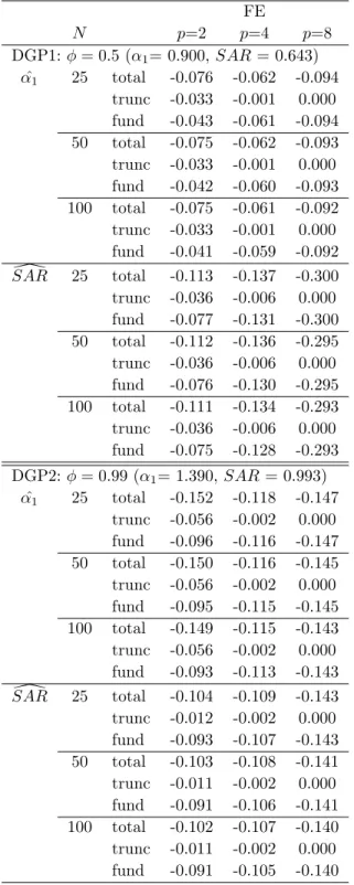
Table 2 provides such a decomposition of the finite-sample bias of the FE estimator when the
data are generated from DGP1 and DGP2 with N = {25,50,100} and T = 25. As we expect a
decreasing contribution of the truncation bias as lag length increases, we report the bias
decom-position when the model is estimated usingp={2,4,8}. From the table, we observe that the FE
estimator suffers substantially from fundamental bias. An important observation is that there is
a tradeoff in the value of p such that, as p increases, the truncation bias vanishes quickly but the
5
Empirical Applications
In this section, we apply our procedure to a panel dataset of micro price series. Our data
are from the American Chamber of Commerce Researchers Association (ACCRA) Cost of Living
Index produced by the Council of Community and Economic Research. Using the individual good
price series from the same data source, Parsley and Wei (1996) and Crucini, Shintani and Tsuruga
(2015) estimate the speed of price adjustment toward the long-run law of one price (LOP) across
US city pairs in terms of the sum of the AR coefficients (SAR). Here, we estimate the SAR using
the dynamic panel estimators by assuming that the rate of convergence is common within the
same category of goods. To this end, we construct 11 panels of quarterly Consumer-Price-Index
(CPI) categorized good price series over 18 years from 1990Q1 to 2007Q4 (T = 72). In measuring
the LOP deviations for each categorized good, we follow Parsley and Wei (1996) and use one
benchmark city out of 52 cities to compute intercity price differentials over time (our benchmark
city is Albuquerque). LetPit and P0tbe the price of a good in city i and that for the benchmark
city, respectively. Then, the LOP deviations are computed asyit= logPit−logP0tfori= 1, ...,51.
As we pool all the goods in the same category, the total number of cross-sectional observations (N)
will be multiples of 51. All the names of individual goods in our categorization are presented in
Table 3.
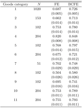
Table 4 reports the estimated sum of the AR coefficients (SAR) for each categorized good
using the FE estimator and the BCFE estimator. We use lags selected by sequential rule with the
maximum lag set at p= 11 based on the formula pmax = [12(T /100)1/4]. The difference between
the FE estimator and the BCFE estimator implies a nonnegligible downward bias.
6
Conclusion
In this paper, we consider the estimation of a dynamic panel autoregressive (AR) process of
by letting the order of the AR process of the fitted model increase with the sample size. We study
the asymptotic properties of the FE estimator and also investigate their finite-sample properties
in simulations. The results indicate that the FE estimator suffers severely from bias, and is not
recommended. The bias-corrected estimator is preferred in terms of the mean squared errors.
Our results are useful for making statistical inferences regarding quantities that are important
in understanding the dynamic nature of an economic variable, such as the long-run effects, without
relying on strong assumptions. Although not discussed in this paper, further applications of our
results are possible. For example, our estimators would be useful in constructing a model-free
impulse response function. See, e.g., Jord`a (2005) and Chang and Sakata (2007) for model-free
impulse response functions in time series analysis. It would also be interesting to extend the
tests of Granger causality by L¨utkepohl and Poskitt (1996) that are based on infinite order AR
models to panel data. Other applications of an AR model of infinite order would be long-run
variance estimation, spectral density estimation and unit root tests. These applications represent
a promising future research agenda.
Appendix
This appendix presents the proofs of Theorems 1, 2, 3 and 4. The proofs of the other theorems
and most of the lemmas are presented in the supplemental materials.
Throughout the appendix, C ∈ (1,∞) denotes a generic bounded constant, which does not
depend on any index and whose actual value varies across occasions. Given a matrixA, we let||A||
denote the Euclidean matrix norm defined by ||A||2 =tr(A′A). Also let||A||
1 denote the Banach
norm so that||A||1 = supx6=0{||Ax||/||x||}, using the Euclidean norm for the vectorl,||l||= (l′l)1/2.
For any symmetric matrix A, we let λmin(A) and λmax(A) be the minimum and the maximum
eigenvalues of A, respectively. We note that ||A||1 = p
positive definite,||A||1=λmax(A). Define γk=E(witwi,t−k). We let
¯
wi,t,τ =
1
τ−t+ 1(wi,t+· · ·+wi,τ).
We also define ¯wi,t,τ(p) = ( ¯wi,t,τ, . . . ,w¯i,t−p+1,τ−p+1)′, ¯wt,τ = ( ¯w1,t,τ, . . . ,w¯N,t,τ)′ and ¯wt,τ(p) =
( ¯wt,τ, . . . ,wt¯−p+1,τ−p+1). Similarly, define ¯ǫi,t,τ = (ǫi,t+· · ·+ǫi,τ)/(τ−t+1) and ¯ǫt,τ = (¯ǫ1,t,τ, . . . ,ǫN,t,τ¯ )′.
LetTp =T−p. Note that Tp =O(T) if p/T →0.
The following inequalities will be used below: ||A||1 = p
λmax(A′A) ≤ (tr(A′A))1/2 = ||A||.
||AB||2 ≤ ||A||2
1||B||2 and ||AB||2 ≤ ||A||2||B||21 (See Lewis and Reinsel (1985) and Wiener and
Masani (1958)). For any conformable matrices A and D and any square matrix B, ||A′BD|| ≤
kBk1||A|| · ||D||.
We repeatedly use the result that there exists C1>0 such that the minimum eigenvalue of Γp
is greater than C1 for any pand there existsC2 <∞ such that the the maximum eigenvalue of Γp
is smaller thanC2 for anyp. This result holds under Assumption 1(iii) by Corollary 3.3 (i) and (ii)
of Davies (1973).
The following lemma is based on the arguments in the proof of Lewis and Reinsel (1985, Theorem
1) or Berk (1974, Lemma 3).
Lemma A.1. Suppose that Assumption 1 is satisfied. Let Γˆp be an estimator of Γp such that
Γˆp−Γp
=Op(ρN,T,p) where ρN,T,p=o(1) as N → ∞, T → ∞ and p → ∞. Then, asN → ∞,
T → ∞ and p → ∞, we have ||Γˆp −Γp||1 = Op(ρN,T,p), ||(ˆΓp)−1 −Γp−1||1 = Op(ρN,T,p) and
and ||(ˆΓp)−1||1 =Op(1).
Let ˜bt,p =bt,p−PTt′=p+1bt′,p/Tp and ˜ǫt=ǫt−¯ǫp+1,T. The estimation error of the FE estimator
can be decomposed as
ˆ
where
ˆ
ΓFp = 1
N Tp T X
t=p+1
˜
xt(p)′x˜t(p), F1 =
1
N Tp T X
t=p+1
˜
xt(p)′˜bt,p and F2=
1
N Tp T X
t=p+1
˜
xt(p)′˜ǫt.
Note that we can write
˜
xt(p) =wt−1(p)−w¯p,T−1(p).
Lemma A.2. Suppose that Assumption 1 is satisfied. If N → ∞, T → ∞ and p → ∞ with
p/T →0, then ||ΓˆF
p −Γp||=Op
p/(pTmin(N, T)).
Lemma A.3. Suppose that Assumption 1 is satisfied. If N → ∞, T → ∞ and p → ∞, then
||F1||=Op √
pP∞k=p+1|αk|
=op(1). In addition, if p2/Tmin(N, T)→0, then ||ℓ′p(ˆΓFp)−1F1||=
OpP∞k=p+1|αk|
.
Lemma A.4. Suppose that Assumption 1 is satisfied. IfN → ∞,T → ∞ andp→ ∞withp/T →
0, we havekBk=O √p,N−1w¯p,T−1(p)′¯ǫp+1,T=Op √p/TandN−1w¯p,T−1(p)′¯ǫp+1,T −B/T=
Op √
p/(√N T).
Proof. We note that
1
Nw¯p,T−1(p) ′ǫ¯
p+1,T =
1
N T2 p
T X
t=p+1 T X
m=p+1
wt−1(p)′ǫm.
We observe that E(wt−1(p)′ǫm) = 0 if t−1 < m. Let ψk(p) = (ψk, . . . , ψk−p+1)′. Since wt−1 = P∞
k=0ψkǫt−1−k, we have E(wt−1(p)′ǫm) =N σ2ψt−1−m(p) ift−1≥m. Thus, we have that
B T =E
1
Nw¯p,T−1(p) ′¯ǫ
p+1,T = 1 T2 p T X
t=p+2 t−1 X
m=p+1
σ2ψt−1−m(p).
We observe that
kBk2 =σ4T 2 T4 p p−1 X k=0 T X
t=p+2 t−1 X
m=p+1
ψt−1−m−k
2
≤σ4T 2 T4 p p−1 X k=0 T X
t=p+2 ∞ X
m=0
|ψm|
2
=O(p). (7)
Next, we examine E 1
Nw¯p,T−1(p) ′¯ǫ
p+1,T − B T 2 = tr var 1
Nw¯p,T−1(p) ′¯ǫ
p+1,T
= 1
Ntr(var( ¯wi,p,T−1(p)¯ǫi,p+1,T))
= 1
N p−1 X
k=0
var( ¯wi,p−k,T−1−k¯ǫi,p+1,T).
We also see that
var( ¯wi,p−k,T−1−k¯ǫi,p+1,T) ≤ E( ¯w2i,p−k,T−1−kǫ¯2i,p+1,T)
≤ qE( ¯w4
i,p−k,T−1−k) q
E(¯ǫ4 i,p+1,T).
It holds that
E( ¯w4i,p−k,T−1−k) = 1
T4 p
T−1−k X
t1=p−k
T−1−k X
t2=p−k
T−1−k X
t3=p−k
T−1−k X
t4=p−k
E(wi,t1wi,t2wi,t3wi,t4)
= 3
T4 p
T−1−k
X
t1=p−k
T−1−k X
t2=p−k
E(wi,t1wi,t2)
2 + 1 T4 p
T−1−k X
t1=p−k
T−1−k X
t2=p−k
T−1−k X
t3=p−k
T−1−k X
t4=p−k
κw(t1, t2, t3, t4) =O
1
T2
by Assumption 1. Moreover,
E(¯ǫ4i,p+1,T) = 1
T4 p
((T−p)E(ǫ4it) + 3Tp(Tp−1)σ4) =O
1
T2
.
It therefore follows that
E 1
Nw¯p,T−1(p) ′¯ǫ
p+1,T − B T 2
=O 1 N p−1 X k=0 r 1 T2 1 T2 !
=O p N T2
. (8)
Therefore, the Chebyshev inequality shows that
1
Nw¯p,T−1(p) ′¯ǫ
p+1,T − B T =Op
√p
√
N T
.
Lastly, by (8) and (7), we have
E 1
Nw¯p,T−1(p) ′ǫ¯
p+1,T 2 = tr var 1
Nw¯p,T−1(p) ′¯ǫ
p+1,T
+ 1
T2tr BB ′
= O p N T2
+O p T2
=O p T2
The Chebyshev inequality gives
1
Nw¯p,T−1(p) ′¯ǫ
p+1,T =Op
√p
T
.
Lemma A.5. Suppose that Assumption 1 is satisfied. IfN → ∞,T → ∞ andp→ ∞withp/T →
0, then ||F2||=Op p
p/(Tmin(N, T))=op(1) and ||F2+B/T||=Op p
p/(N T)=op(1).
Lemma A.6. Suppose that Assumption 1 is satisfied. If N → ∞, T → ∞ and p → ∞ with
p3/(N T)→0 and p/T →0, then pN Tpℓp′Γ−1p (F2+B/T)/vp →dN(0,1).
Proof of Theorem 1
Proof. We have
||αˆF(p)−α(p)||=||(ˆΓFp)−1(F1+F2)|| ≤ ||(ˆΓFp)−1||1||F1||+||(ˆΓFp)−1||1||F2||.
Lemmas A.1 and A.2 give that ||(ˆΓFp)−1||1 =Op(1). Lemma A.3 gives that ||F1|| =op(1). Lastly,
||F2||=op(1) follows by Lemma A.5.
Proof of Theorem 2
Proof. We note that
p
N Tp(ℓ′pαˆF(p)−ℓ′pα(p) +ℓ′pΓ−1p B/T)
= pN Tpℓ′p(ˆΓFp)−1F1+ p
N Tpℓ′p(ˆΓFp)−1F2+ p
N Tpℓ′pΓ−1p B/T
= pN Tpℓ′p(ˆΓFp)−1F1+ p
N Tpℓ′p((ˆΓFp)−1−Γ−1p )F2+ p
N Tpℓ′pΓ−1p (F2+B/T).
Lemma A.3 states that the first term is of orderop(1) by the assumption of the theorem. Lemma A.6
gives that the third term is asymptotically standard normal. Note that p3N/(Tmin(N2, T2))→0
implies p3/(N T)→0 andp/T →0.
We now consider the second term. We see that
We have ||ℓp||1 = O(1), ||(ˆΓFp)−1 −Γˆ−1p ||1 = Op(p/( p
Tmin(N, T))) by Lemmas A.1 and A.2
and ||pN TpF2|| =Op( p
pN/min(T, N)) by Lemma A.5. Therefore, we have ||√N T ℓ′
p((ˆΓFp)−1−
Γ−1p )F2||=Op(p3/2
√
N /(√Tmin(N, T))), which is op(1) under the assumption of the theorem.
Proof of Theorem 3
Before presenting the proof, we provides a lemma that gives the rate of convergence of the bias
estimator.
Lemma A.7. Suppose that Assumption 1 is satisfied. Then if N → ∞, T → ∞, andp→ ∞ with
p2/(Tmin(N, T))→0, we have
kBˆ−Bk=op(T).
If N → ∞, T → ∞, and p→ ∞ with √N TP∞k=p+1|αk| → 0, p3/(Tmin(N, T))→ 0, p2/T → 0,
and p3N/(Tmin(N2, T2))→0, We have
kBˆ−Bk=Op p p Tmin(N, T)
!
.
Proof. We first approximate B byT(σ2P∞k=0ψk/(T−p))ι=T(σ2/((1−Ppk=1αk)(T−p))ιp. The
rth element ofψt−1−m(p) isψt−m−r. Thus, therth element ofB is
T
(T−p)2 T X
t=p+2 t−1 X
m=p+1
σ2ψt−m−r = T σ2
(T −p)2
T−p−r−1 X
k=0
(T −p−r−k)ψk.
The difference between thekth element ofB/T and σ2P∞
k=0ψk/(T −p) is
σ2
(T−p)2
T−p−r−1 X
k=0
(T −p−r−k)ψk−
1
T −pσ 2
∞ X
k=0 ψk
=− σ
2
(T−p)2
T−p−r−1 X
k=0
(r+k)ψk− 1 T −pσ
2 ∞ X
k=T−p−r−1 ψk
=− σ
2
(T−p)2 p X
k=0
(r+k)ψk σ2
(T−p)2
T−p−r−1 X
k=p+1
(r+k)ψk−
1
T −pσ 2
∞ X
Noting that √N T P∞k=p+1|αk| →0 implies
√
N T P∞k=p+1|ψk| →0, this difference is of order
O
1
T2 +
1
T√N T
.
Thus the difference betweenB/T and (σ2P∞k=0ψk/(T −p))ι is of order
O √p
T2 +
√p
T√N T
=O
√p
T3/2pmin(N, T) !
.
Next, we evaluate the order of the difference between ˆB/T and (σ2P∞k=0ψk/(T −p))ι =
(σ2/((1−Pkp=1αk)(T−p))ιp. Under the assumption of Theorem 1, we havePpk=1α˜k−Ppk=1αk=
op(√p). Therefore, we have
σ2
1−Ppk=1α˜k ιp
1
T −p −
σ2
1−P∞k=1αk ιp
1
T −p =op
√p
T
√p+ 1
√
N T
=op(1).
This implies thatkBˆ−Bk=op(T). If the assumptions for Theorem 2 are satisfied, we have
p X
k=1
˜
αk− p X
k=1
αk=Op r
p N T +
√p
T
.
We note thatPpk=1αk−P∞k=1αk =−P∞k=p+1αk. Therefore, we have
σ2
1−Ppk=1α˜k ιp
1
T −p −
σ2
1−P∞k=1αk ιp
1
T −p =Op
√p
T r
p N T +
√p T + 1 √ N T
=Op
p
T3/2pmin(N, T) !
.
Thus, we have the desired result.
We now proceed the proof of Theorem 3
Proof. We have
||αˆBF(p)−α(p)|| = ||(ˆΓFp)−1(F1+F2+ ˆB/T)||
≤ ||(ˆΓFp)−1||1(||F1||+||F2+B/T||+||Bˆ−B||/T).
Lemmas A.1 and A.2 give that ||(ˆΓF
p)−1||1 = Op(1). Lemma A.3 gives that ||F1|| = op(1). By
Lemma A.5, we have ||F2 +B/T|| = Op( p
p/(N T))) = op(1). Lemma A.7 gives ||Bˆ −B|| =
Proof of Theorem 4
Proof. We note that
p
N Tp(ℓ′pαˆBF(p)−ℓ′pα(p)) = p
N Tpℓ′p(ˆΓFp)−1(F1+F2+ ˆB/T)
= pN Tpℓ′p(ˆΓFp)−1F1+ p
N Tpℓ′p((ˆΓFp)−1−Γ−1p )(F2+B/T)
+pN Tpℓ′pΓ−1p (F2+B/T) + p
N Tpℓ′p(ˆΓFp)−1( ˆB−B/T).
Similarly to the proof of Theorem 2, we have pN Tpℓ′pΓ−1p (F2+B/T)/vp →d N(0,1) by Lemma
A.6 and||pN Tpℓ′p(ˆΓpF)−1F1||=op(1) by Lemma A.3. We also have
||pN Tpℓ′p((ˆΓpF)−1−Γ−1p )(F2+B/T)|| ≤ ||ℓp||1||(ˆΓpF)−1−Γ−1p ||1|| p
N Tp(F2+B/T)||.
We have ||ℓp||1 = O(1), ||(ˆΓFp)−1 −Γˆ−1p ||1 = Op(p/ p
Tmin(N, T)) by Lemmas A.1 and A.2 and
||√N T(F2+B/T)||=Op(√p) by Lemma A.5. Therefore, we have ||pN Tpℓ′p((ˆΓFp)−1−Γ−1p )(F2+
B/T)||=Op(p3/2/ p
Tmin(N, T)), which isop(1) under the assumption of the theorem. Lastly, by
Lemma A.7, we have
||pN Tpℓ′p(ˆΓFp)−1( ˆB−B)/T|| ≤||ℓp||1||(ˆΓFp)−1||1|| p
N Tp( ˆB−B)/T||
=Op
p√N Tpmin(N, T)
!
=op(1).
References
Alvarez, J. and Arellano, M. (2003). The time series and cross-section asymptotics of dynamic panel data estimators,Econometrica 71(4): 1121–1159.
Berk, K. N. (1974). Consistent autoregressive spectral estimates,Annals of Statistics2(3): 489–502.
Chang, P.-L. and Sakata, S. (2007). Estimation of impulse response functions using long autore-gression,Econometrics Journal 10: 453–469.
Crucini, M. J., Shintani, M. and Tsuruga, T. (2015). Noisy information, distance and law of one price dynamics across US cities,Journal of Monetary Economics 74: 52–66.
Franco, F. and Philippon, T. (2007) Firms and aggregate dynamics,The Review of Economics and Statistics 89(4): 587–600.
Gon¸calves, S. and Kilian, L. (2007). Asymptotic and bootstrap inference for AR(∞) processes with conditional heteroskedasticity,Econometric Reviews 26(6): 609–641.
Hahn, J. and Kuersteiner, G. (2002). Asymptotically unbiased inference for a dynamic panel model with fixed effects when bothn and T are large, Econometrica 70(4): 1639–1657.
Hahn, J. and Newey, W. (2004). Jackknife and analytical bias reduction for nonlinear panel models, Econometrica 72(4): 1295–1319.
Han, C., Phillips, P. C. B. and Sul, D. (2014). X-differencing and dynamic panel model estimation, Econometric Theory 30: 201–251.
Hannan, E. J. and Deistler, M. (1988). The Statistical Theory of Linear Systems, John Wiley & Sons, Inc., New York.
Hayakawa, K. (2009). A simple efficient instrumental variable estimator for panel AR(p) models when bothN and T are large, Econometric Theory 25: 873–890.
Hayashi, F. (2000). Econometrics, Princeton University Press, Princeton.
Head, A., Lloyd-Ellis, H. and Sun, H. (2014). Search, liquidity, and the dynamics of house prices and construction,American Economic Review 104(4): 1172–1210.
Jord`a, O. (2005). Estimation and inference of impulse responses by local projections, American Economic Review 95(1): 161–182.
Kiviet, J. F. (1995). On bias, inconsistency, and efficiency of various estimators in dynamic panel data models, Journal of Econometrics 68: 53–78.
Kuersteiner, G.M. (2005). Automatic inference for infinite order vector autoregressions, Economet-ric Theory 21: 85–115.
Lee, Y. (2006).General Approaches to Dynamic Panel Modelling and Bias Correction, Ph.D. thesis, Yale University.
Lee, Y. (2012). Bias in dynamic panel models under time series misspecification,Journal of Econo-metrics 169: 54–60.
Lee, Y. and Phillips, P. C. B. (2015). Model selection in the presence of incidental parameters, Journal of Econometrics,188: 474–489.
Lewis, R. and Reinsel, G. C. (1985). Prediction of multivariate time series by autoregressive model fitting,Journal of Multivariate Analysis 16: 393–411.
L¨utkepohl, H. and Poskitt, D. S. (1991). Estimating orthogonal impulse responses via vector autoregressive models,Econometric Theory 7: 487–496.
L¨utkepohl, H. and Poskitt, D. S. (1996). Testing for causation using infinite order vector autore-gressive processes,Econometric Theory 12: 61–87.
L¨utkepohl, H. and Saikkonen, P. (1997). Impulse response analysis in infinite order vector autore-gression processes,Journal of Econometrics 81: 127–157.
Neyman, J. and Scott, E. L. (1948). Consistent estimates based on partially consistent observations, Econometrica 16: 1–32.
Nickell, S. (1981). Biases in dynamic models with fixed effects, Econometrica 49(6): 1417–1426.
Okui, R. (2010). Asymptotically unbiased estimation of autocovariances and autocorrelations with long panel data, Econometric Theory 26: 1263–1304.
Parsley, D. C. and Wei, S.-J. (1996). Convergence to the law of one price without trade barriers or currency fluctuations,Quarterly Journal of Economics 111(4): 1211–1236.
Phillips, P. C. B. and Moon, H. R. (1999). Linear regression limit theory for nonstationary panel data, Econometrica 67(5): 1057–1111.
Table 1: Finite sample performance of estimators whenN=100
FE BCFE
T=25 50 100 T=25 50 100
DGP1:φ= 0.5 (α1= 0.900,SAR= 0.643)
automatic pˆ mean 7.68 8.91 9.70 5.03 6.06 7.20 lag αˆ1 RMSE 0.093 0.035 0.017 0.033 0.017 0.011
mean bias -0.089 -0.031 -0.013 -0.021 -0.005 -0.001 st dev 0.026 0.016 0.011 0.026 0.016 0.011 cp 0.055 0.493 0.766 0.815 0.927 0.944 [
SAR RMSE 0.288 0.125 0.060 0.067 0.032 0.018 mean bias -0.283 -0.121 -0.057 -0.060 -0.026 -0.012 st dev 0.052 0.031 0.019 0.030 0.019 0.013 cp 0.000 0.001 0.032 0.383 0.666 0.819 fixed pˆ mean 8 10 12 8 10 12 lag αˆ1 RMSE 0.095 0.036 0.017 0.045 0.018 0.011
mean bias -0.092 -0.033 -0.013 -0.036 -0.008 -0.002 st dev 0.026 0.016 0.011 0.026 0.016 0.011 cp 0.047 0.468 0.758 0.662 0.909 0.943 [
SAR RMSE 0.297 0.133 0.066 0.090 0.039 0.020 mean bias -0.293 -0.131 -0.064 -0.085 -0.033 -0.014 st dev 0.044 0.026 0.017 0.030 0.021 0.015 cp 0.000 0.000 0.018 0.353 0.740 0.882 DGP2:φ= 0.99 (α1= 1.390,SAR= 0.993)
automatic pˆ mean 5.52 7.19 8.63 7.11 7.32 7.74 lag αˆ1 RMSE 0.128 0.057 0.026 0.084 0.035 0.016
mean bias -0.125 -0.055 -0.023 -0.080 -0.031 -0.012 st dev 0.027 0.016 0.011 0.026 0.016 0.011 cp 0.001 0.060 0.403 0.101 0.480 0.780 [
SAR RMSE 0.123 0.055 0.024 0.091 0.044 0.021 mean bias -0.121 -0.054 -0.024 -0.090 -0.044 -0.021 st dev 0.021 0.008 0.003 0.011 0.005 0.003 cp 0.000 0.000 0.000 0.000 0.000 0.000 fixed pˆ mean 8 10 12 8 10 12 lag αˆ1 RMSE 0.146 0.061 0.027 0.089 0.038 0.017
mean bias -0.143 -0.059 -0.024 -0.085 -0.034 -0.013 st dev 0.026 0.017 0.011 0.027 0.017 0.011 cp 0.000 0.045 0.383 0.080 0.429 0.762 [
SAR RMSE 0.141 0.059 0.026 0.094 0.046 0.022 mean bias -0.140 -0.059 -0.026 -0.093 -0.046 -0.022 st dev 0.018 0.007 0.003 0.012 0.006 0.003 cp 0.000 0.000 0.000 0.000 0.000 0.000
Table 2: Decomposition of the finite sample bias of FE estimator whenT = 25
FE
N p=2 p=4 p=8
DGP1:φ= 0.5 (α1= 0.900,SAR= 0.643) ˆ
α1 25 total -0.076 -0.062 -0.094 trunc -0.033 -0.001 0.000 fund -0.043 -0.061 -0.094 50 total -0.075 -0.062 -0.093 trunc -0.033 -0.001 0.000 fund -0.042 -0.060 -0.093 100 total -0.075 -0.061 -0.092 trunc -0.033 -0.001 0.000 fund -0.041 -0.059 -0.092 [
SAR 25 total -0.113 -0.137 -0.300 trunc -0.036 -0.006 0.000 fund -0.077 -0.131 -0.300 50 total -0.112 -0.136 -0.295 trunc -0.036 -0.006 0.000 fund -0.076 -0.130 -0.295 100 total -0.111 -0.134 -0.293 trunc -0.036 -0.006 0.000 fund -0.075 -0.128 -0.293 DGP2:φ= 0.99 (α1= 1.390,SAR= 0.993)
ˆ
α1 25 total -0.152 -0.118 -0.147 trunc -0.056 -0.002 0.000 fund -0.096 -0.116 -0.147 50 total -0.150 -0.116 -0.145 trunc -0.056 -0.002 0.000 fund -0.095 -0.115 -0.145 100 total -0.149 -0.115 -0.143 trunc -0.056 -0.002 0.000 fund -0.093 -0.113 -0.143 [
SAR 25 total -0.104 -0.109 -0.143 trunc -0.012 -0.002 0.000 fund -0.093 -0.107 -0.143 50 total -0.103 -0.108 -0.141 trunc -0.011 -0.002 0.000 fund -0.091 -0.106 -0.141 100 total -0.102 -0.107 -0.140 trunc -0.011 -0.002 0.000 fund -0.091 -0.105 -0.140
Table 3: List of goods
CPI categorization ACCRA categorization
1 Food at home T-bone steak, Ground beef, Frying chicken, Chunk light tuna, Whole milk, Eggs, Margarine, Parmesan cheese, Potatoes, Bananas, Lettuce, Bread, Coffee, Sugar, Corn flakes, Sweat peas, Peaches, Shortening, Frozen corn, Soft drink
2 Food away from home Hamburger sandwich, Pizza, Fried chicken
3 Alcoholic beverages Beer, Wine
4 Shelter Apartment, Home purchase price, Mortgage rate, Monthly payment
5 Fuel and other utilities Total home energy cost, Telephone
6 Household furnishings Facial tissues, Dishwashing powder, Dry cleaning, and operations Major appliance repair
7 Men’s and boy’s apparel Men’s dress shirt
8 Private transportation Auto maintenance, Gasoline
9 Medical care Doctor office visit, Dentist office visit
10 Personal care Haircut, Beauty salon, Toothpaste, Shampoo
11 Entertainment Newspaper subscription, Movie, Bowling, Tennis balls
Table 4: Sum of the AR coefficients estimates
Goods category N FE BCFE 1 1020 0.687 0.726
(0.005) (0.005) 2 153 0.662 0.713
(0.014) (0.014) 3 102 0.753 0.780
(0.014) (0.014) 4 204 0.820 0.848
(0.008) (0.008) 5 102 0.768 0.797
(0.014) (0.015) 6 204 0.675 0.721
(0.012) (0.012)
7 51 0.702 0.748
(0.029) (0.029) 8 102 0.504 0.580
(0.026) (0.026) 9 102 0.695 0.741
(0.016) (0.016) 10 204 0.753 0.789
(0.011) (0.011) 11 204 0.755 0.793
(0.011) (0.011)