MarkovSwitching VAR approach Research Hiroshi Morita's Homepage

(1)

H i-S tat D isc us sion P ap er

Research Unit for Statistical

and Empirical Analysis in Social Sciences (Hi-Stat)

Hi-Stat

Institute of Economic Research Hitotsubashi University 2-1 Naka, Kunitatchi Tokyo, 186-8601 Japan

Global COE Hi-Stat Discussion Paper Series

Research Unit for Statistical

and Empirical Analysis in Social Sciences (Hi-Stat)

January 2013

Regime Switches in Japanese Fiscal Policy:

Markov-Switching VAR Approach

Jun-Hyung Ko

Hiroshi Morita

270

(2)

Regime Switches in Japanese Fiscal Policy:

Markov-Switching VAR Approach

JUN-HYUNG KO

^†

and HIROSHI MORITA

^‡

†

University of Tokyo

^‡

Hitotsubashi University

December, 2012

Abstract

This paper empirically investigates the changing dynamics of fiscal policy shocks to the macroeconomy in Japan. By estimating a Markov-switching vector-autoregressive (VAR) model, regime switches in both automatic fiscal responses to output and discretionary fiscal shocks are investigated. The main findings are summarized as follows. First, the best-fit model is a version with four regimes that allows time variation in both coefficients and disturbance variances. Second, the structural changes occurred in the mid-1970s, the early 1990s, and the late 1990s. Third, in contrast to the other regimes, expansionary fiscal shocks depress output and consumption in the third regime. Fourth, fiscal shocks crowd out investment only in the fourth regime. Fifth, the twin-deficit hypothesis holds in all regimes.

Keywords: fiscal policy, twin-deficit hypothesis, Markov-switching, VAR JEL classification: C11; C32; E62

(3)

1 Introduction

This paper examines the time-varying effects of fiscal shocks on the macroeconomy in Japan. The Japanese economy is useful for this investigation because Japan has already experienced what US and European economies are currently experiencing. First, the Japanese economy experienced a bubble with a steep increase of housing and real state prices from the late 1980s to the early 1990s, which was accompanied by a deep and prolonged recession in the 1990s. Second, tremendous volumes of government stimulus packages were poured into the staggering economy. Third, Japan fell into the so-called liquidity trap at the zero nominal interest rate from the late 1990s to the early 2000s.

A growing number of empirical papers investigate whether the effect of fiscal policy in Japan has changed or even vanished since the 1990s. For example, Ihori, Nakazato, and Kawade (2003) divide the sample period into pre-1990 and post-1990 periods and find that increasing public investment in the 1990s crowded out private investment to some extent and did not substantially increase private consumption. Using a VAR event study approach, Miyazaki (2010) examines the effects of fiscal policy in the 1990s and finds that the negative effect of fiscal policy in the late 1990s was larger and more persistent. Estimating Blanchard-Perotti-type VAR, Watanabe, Yabu, and Ito (2009) find that the government spending shock lost its effect on output in the second subsample period, starting from the late 1980s. Extending their work and incorporating the debt feedback rule, Ko and Morita (2011) also find a similar result.¹ Performing a Bayesian estimation of a dynamic stochastic general equilibrium (DSGE) model, Eguchi (2012) also finds that public spending in the 1990s was less effective. However, these previous works share a common caveat: the timing of structural changes is exogenously imposed. A natural question is how, endogenously permitting the structural changes in the empirical model, we can identify pure fiscal shocks.

We contribute to the existing literature on the above-mentioned question by estimating a multivariate Markov-switching VAR (MS-VAR) model for fiscal policy. Standard VAR models are generally linear systems but the Japanese economy during our sample period experienced many distinctive eras including a high growth period, an unprece- dented bubble and bust, a prolonged recession, and a slight recovery. For this reason, we need to detect possible structural shifts and estimate the VAR model for each sub-sample period. The novelty in this paper lies in the estimation of structural shifts and the parameters for each regime in a single model.² In this respect, we estimate several versions of VAR models with various combinations of time-varying or time-invariant coefficients and variances and compare which version fits the data best.³ In terms of regime shifts, we consider the case where regime changes are to be monotonic, and hence old regimes are to be constrained from occurring again. However, we do not consider too many numbers of regime changes because the number of structural changes of fiscal policy shocks are thought to be limited during our sample period, and we empirically face the problem of the degree of freedom when we derive the impulse response functions. Consequently, one

1Ko and Morita (2011) emphasize that the accumulating government debt should be considered in estimating the effect of government spending shocks. Morita (2012) considers the implementation lag, which is a time lag implementing government expenditure after the fiscal authority decides to spend.

2Two exceptions are Kameda (2011), who estimates a threshold VAR model, and Shioji (2012), who estimates a time-varying VAR model.

3We compare the log marginal likelihood, which is common in the Bayesian literature.

(4)

to four regimes are considered.

Our regime switching methodology is independent of a particular assumption of fiscal shock identification in the fiscal VAR literature.⁴ We adopt the method of Blanchard and Perotti (2002) to identify pure fiscal shocks. The key assumption is the automatic responses of taxes and spending to output. In the case of spending, decision and implementation lags in the political process take presumably more than one quarter and hence government spending cannot respond discretionarily to the unexpected events. For taxes, it has a “built-in stabilizer” effect: when the economy is in a boom, tax revenues increase and vice versa. To identify purely discretionary fiscal shocks, we disentangle these automatic responses to taxes and spending to economic activity using institutional information about the tax and transfer systems. A new element of this paper is that we permit these automatic adjustments of taxes and discretionary fiscal policy to change in each regime.

The main findings in this paper are as follows. First, we find that the best-fit model is the four-regime model that permits changes both in coefficients and variances. Second, under the four-regime model, we find that the regime switches occurred in the mid-1970s, the early 1990s, and the late 1990s. In other words, the estimated periods of the four regimes are (a) the high growth period until the mid-1970s, (b) a stable macroeconomic period from the mid 1970s to the late 1980s and the bubble period that lasted until the early 1990s, (c) the deep recession from the early 1990s to the late 1990s, and (d) the prolonged recession from the late 1990s and the recovery in the early 2000s. Third, the impulse response functions reveal that the sign and significance of the output response are quite different among regimes. In the first two regimes, government spending shocks are found to be persistently effective in increasing output. In particular, in the second regime, the period from the end of the first oil crisis to the beginning of the recession after the bubble burst, the Japanese economy enjoyed the most favorable and statistically significant effect of the fiscal shocks. We also observe a positive effect on output in the fourth regime but the effect is very short-lived. In the third regime, however, the effect on output becomes negative both in the short run and the long run. Fourth, forecast error variance decomposition reveals that government spending shocks appear to play an important role in the first regime while tax shocks explain a large share of output variance in the third regime.

Next, extending our benchmark findings, we also assess the fiscal effect on the other macro variables following two strands of existing fiscal literature. The first strand focuses on the fiscal effect on consumption because the theoretical implications are still inconclu- sive. For example, the traditional Hicksian IS-LM model predicts that the expansionary fiscal shocks crowd in private consumption, while the standard real business cycle models predict that consumption declines. The second strand investigates the “twin-deficit” hypothesis, which asserts that the fiscal deficit leads to a deterioration of trade balances. A number of empirical studies find that the twin-deficit hypothesis holds in US and Eu- ropean economies, while this hypothesis has not been fully investigated in Japan.⁵ Three

4See, for example, the institutional information approach in Blanchard and Perotti (2002), the sign- restriction approach in Mountford and Uhlig (2009) and Fisher and Peters (2010), and the narrative- record approach in Ramey (2011) and Romer and Romer (2010), among others.

5See, for example, Monacelli and Perotti (2010), Corsetti, Meier, and M¨uller (2009), and Ravn, Schmitt-Groh´e, and Uribe (2007) for the US economy, and Beetsma, Klaassen, and Giuliodori (2008) and Castro and Garrote (2012) for the Euro area, among others.

(5)

more findings are as follows. First, we observe the contractionary effect on consumption of lax fiscal stimuli in the third regime. Second, in the second regime, expansionary fiscal shocks significantly crowd in private investment, which contributes to the significant increase of output. In contrast, we find the “investment crowding out” effect in the fourth regime. Third, in all regimes, fiscal deficit shocks with spending lead to trade balance deterioration. This result in Japan is in line with the twin-deficit hypothesis.⁶

The remainder of the paper is organized as follows. Section 2 describes the MS-VAR model and the identification scheme. Section 3 compares the empirical models. Section 4 displays the main results. Section 5 shows the results of the 4-variable VAR with consumption and investment. Section 6 investigates the twin-deficit hypothesis. Section 7 concludes the paper.

2 Estimation methodology

2.1 Markov-switching VAR model

We estimate the following MS-VAR model with Blanchard and Perotti (2002) type identification:

Yt _{= C}0_(s_t_{) + C}1_(s_t_)Yt

−¹+ · · · + C^M(st)Y^t₋^M + u^t, ut ∼ N (0, Σ(st)), (1)

A(st)u^t = B(st)ε^t, (2)

where Y^t = [∆gt^,∆τt^,∆yt]^′is a (3×1) vector that consists of government expenditure, tax revenue, and output in log-difference forms. C0(s_t) is a vector of constants. C^m(s_t) where m∈ {1, · · · , M } is a matrix with coefficients. u^tis a vector of reduced-form residuals with a variance-covariance matrix denoted by Σ(st). ε^t is a vector of structural shocks that are mutually independent. Moreover, s_t = 1, 2, · · · , S is the latent variable representing a regime in period t, where S is the number of regimes. We assume its evolution follows a Markov process. For example, in the case that we assume an absorbing two-state model, the regime changes according to the following transition probability matrix P :

P =

[ p₁₁ 0 1 − p11 1 ]

, (3)

where the (i, j) element of P indicates P r[st= i | s_t−1= j].

As in Ito, Watanabe, and Yabu (2011) and Inoue and Okimoto (2008), we estimate this model via the Bayesian method. More precisely, the Gibbs sampler is adopted among the Markov chain Monte Carlo (MCMC) methods. A brief explanation of estimation process is as follows.⁷ Firstly, we define ˜Y = {Y^t}^T_t=1, ˜s= {st}^T_t=1, C(st) ≡ [C⁰(st), · · · , C^M(st)] where Cm(st) ≡ [Cm(1), · · · , Cm(S)], Σ(st) ≡ [Σ(1), · · · , Σ(S)], and ˜^p is a component of a transition probability matrix. Secondly, we set the prior distribution for each parameter. This paper chooses the independent Normal-Wishart prior for the vector- ized coefficient matrix and variance-covariance matrix, and the beta distribution for the transition probabilities.⁸

6We also find that the real exchange rate appreciates in the first regime but depreciates in the latter two regimes.

7Kim and Nelson (1999) explain the estimation process in detail.

8Krolzig (1997) describes the posterior distributions for the MS-VAR.

(6)

Given the above settings, we can generate random samples from π(˜^{s, C,}Σ, ˜^p| ˜^Y) as follows.

1. Set initial values in ˜s⁽⁰⁾, C⁽⁰⁾,Σ⁽⁰⁾,p˜⁽⁰⁾ and set j = 0. 2. Generate ˜^s^(j+1) from π(˜^s| C^(j),Σ^(j),^p˜^(j), ˜Y_).

3. Generate ˜p^(j+1) from π( ˜p| C^(j),Σ^(j),s˜^(j+1), ˜Y). 4. Generate C^(j+1) from π(C | Σ^(j),s˜^(j+1),p˜^(j+1), ˜Y). 5. Generate Σ^(j+1) from π(Σ | C^(j+1),^s˜^(j+1),^p˜^(j+1), ˜Y_).

6. Repeat the process from Step 2 to Step 5 using ˜s^(j+1), C^(j+1),Σ^(j+1),p˜^(j+1) as initial values.

We iterate this process N = 30000 times and the first N₀ = 20000 samples are discarded as a burn-in.

2.2 Identification and data

We identify the structural shocks following Blanchard and Perotti (2002). In contrast to the previous literature, we consider the case that each element of the matrices A(st) and B_(s_t) in equation (2) can be changed among regimes as follows:





1 0 a_gy(st) 0 1 a_{τ y}(st) a₃₁(st) a32(st) 1







 u^g_t u^τ_t u^y_t



=





1 0 0

b₂₁(st) 1 0

0 0 1







 ε^g_t ε^τ_t ε^y_t



. (4)

Using the external information, we identify a_gyand a_{τ y}, which represent the automatic fiscal responses to output. The data of these two output elasticities are taken from Watanabe et al. (2009). For the tax elasticity to output, aτ y(st), we use the average value for each estimated regime. The different values of a_{τ y}(s_t) among regimes indicate that both the ratios of individual taxes and transfers to net taxes as well as the tax base elasticities have changed over time. The remaining parameters, a31(st), a32(st), and b₂₁(s_t), are the estimates for each sampled regime. The only exception from time variation is agy(st), the automatic response parameter of government expenditure to output fluctuations. We set agy(st) = 0 for the whole sample period because it is hard to believe that the political process changes among regimes. Hence, the matrices A(s_t) and B(st) depend on the regime when we allow the variance-covariance matrix to be changed.⁹

Data are quarterly and the sample period is 1965Q1-2004Q4. Government spending, tax revenue, and GDP are taken from Watanabe et al. (2009), where government spending is defined as the sum of final consumption expenditure and gross investment of general

9Blanchard-Perotti-type identification has been recently criticized because the implementation lags may obscure the identification and the disentangled stimulus might be a mix of anticipated and unanticipated changes. For example, Ramey (2011) uses the expected discounted value of military expenditures as a proxy to obtain purely unanticipated government shocks. Morita (2012) disentangles anticipated and unanticipated government shocks in Japan using the sign-restriction method developed by Fisher and Peters (2010). We leave this issue for future research.

(7)

and local governments. Private consumption, private investment, exports, and imports are downloaded from the SNA database. 93SNA data starts from 1980Q1, and hence we extend 93SNA data for 1965Q1-1979Q4 using the growth rate of 68SNA. The data source for the exchange rate is the Bank of Japan. The series of a real effective exchange rate starts from 1970Q1, and hence we construct the data before 1970 using the growth rate of a nominal exchange rate against American dollars. All data are real variables. Except for the exchange rate, the series are seasonally adjusted and per capita. In the estimation, all variables are transformed into log-difference forms. Fig.1 shows the data used in the VAR specification.

Fig. 1 is inserted here.

3 Model comparison: transmission mechanism or size

of shocks?

In this section, we explain the model comparison. In the case that the effects of fiscal policy shocks have changed in the Japanese economy, two possible reasons can be considered. One reason is the change of the transmission mechanism of the economy, and the other is that the impact size of the shocks may have changed.¹⁰ Therefore, different from the benchmark case, we consider two other specifications. The first is the case that the coefficient matrix of the independent variables can be changed while the variances of the residuals are assumed to be time-invariant. The second case is that the variances of the residuals can be different among regimes while the coefficient matrix of the independent variables is assumed to be fixed. Estimating monetary VAR models, Sims and Zha (2006) point out that the model with time variation in coefficients reflects the policy regime changes and the nonlinear effects of these changes on private sector dynamics. The structural change of the coefficients of the independent variables indicates that the reaction of dependent variables, such as output to their lags, has changed, and hence may reflect that the transmission mechanism has changed.

We consider the following four cases of restricted time variation for C(st) and Σ(st):¹¹

C(st), Σ(st), A(st), B(st) =











C, ¯¯ _{Σ, ¯}A, ¯B _{Case I} C,¯ Σ(st), A(st), B(st) Case II C(st), ¯Σ, ¯A, ¯B Case III C_(s_t_{), Σ(s}_t_{), A(s}_t_{), B(s}_t_{) Case IV}











(5)

where the bar variable means that this variable is assumed to be constant across time. We set four quarters as the number of lags and assume that this lag length is not time- varying. Case I is an equation with unvarying coefficients and disturbance variances. Case II is an equation with time-varying disturbance variances only, while Case III is an equation with time-varying coefficients only. Case IV is the case that all parameters change.

10This kind of specification is often considered in the time-varying parameter VAR literature. For the US economy, see Cogley and Sargent (2005) and Sims and Zha (2006) among others. For the Japanese economy, Nakajima, Kasuya, and Watanabe (2011) estimate the marginal likelihoods of the time-varying-parameter VAR model and other VAR models for monetary policy.

11This estimation approach is similar to Sims and Zha (2006), who investigate the changing dynamics of monetary policy in the US economy.

(8)

Case II corresponds to the case that the variance of policy shocks in the first two equations and macro shocks in the third equation have changed within the sample period. Case III is the case that the reactions to the lagged variables can change, which reflects the changes of the government’s stance in the first two equations in the VAR model and the transmission of the private economy in the third equation. In the case that we capture only private sector behavior, we may allow the coefficients in the third equation with an output dependent variable to change. The case with time-varying coefficients in the first two equations reflects the possibility that the endogenous reaction of policy-rule dependent variables has changed substantially.

Our estimation is done for up to four possible regimes with three structural changes. Empirically, this is because the system of equations and the number of free parameters become too large. In reality, it is hard to believe that the regimes last only a few years given the fact that the Liberal Democratic Party was the ruling party during the entire sample period.

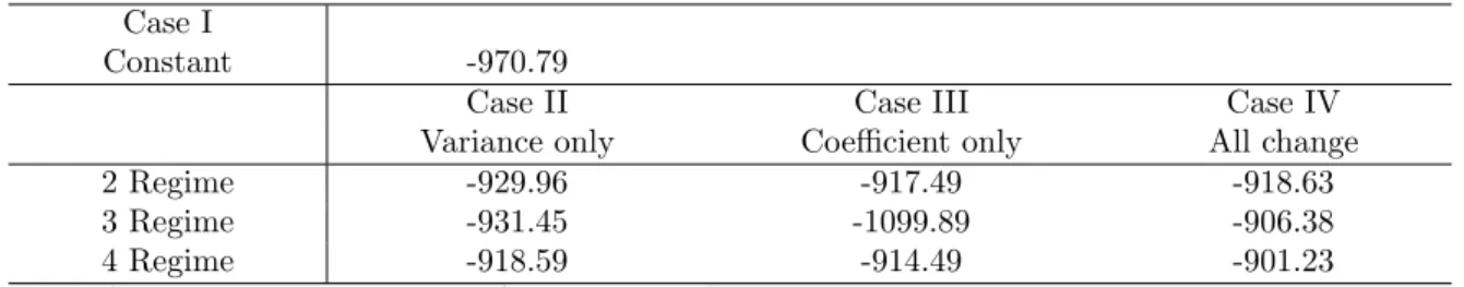
Table 1 displays the model comparison based on log-marginal likelihood. The best fit is for the four-regime “All change” model. Among the “Coefficients only” models and the “Variances only” models, 2 regimes with one structural change in the mid-1970s show the best fit.

Table 1 is inserted here.

4 Main results

4.1 Smoothing probability and impulse responses

In this section, we present the main results from the four-regime “All change” model. We call each regime “Regime i” for i ∈ {1, · · · , 4}. Fig.2 displays the distribution of states by examining the pattern of smoothed probabilities. We observe that Regime 1 switched abruptly around 1975. The timing of this shift is consistent with previous literature such as Ko and Murase (2012).¹² Regime 1 is the period where the Japanese economy maintained high economic growth with a high volume of trade surplus. After the oil crisis, from the mid-1970s to the mid-1980s, the economic situation was very stable, with moderated macro indices such as output and inflation. The volume of social transfers began to rise in the mid-1970s. From the late 1980s to the early 1990s, the Japanese economy experienced a bubble period. After the Plaza Accord, the Japanese income account started to increase because of yen appreciation. Furthermore, there was an investment boom in the domestic market, and government revenue was in at its highest level because of the boom.¹³ Regime 3 starts from the early 1990s and lasts until 1997.¹⁴ Regime 3 is the period where the Japanese economy fell into a deep recession. Although there was a slight recovery in the early 2000s, the whole period of the 1990s and 2000s is often referred to as the Lost Decades.

12For the characteristics of Regime 1, see Ko and Murase (2012).

13For the review of the bubble in the late 1980s and its bursting in the early 1990s, see Ito and Mishkin (2006).

14This timing coincides with the result of Inoue and Okimoto (2008), who investigate the effect of monetary policy.

(9)

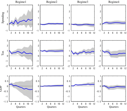
Fig.3 reports the evolution of the estimated impulse responses of each dependent variable to a one-percent government spending shock in the four regimes. For each regime, we collect the impulse responses for 12 periods of the horizons. The solid blue and dotted red lines indicate the posterior mean of sampled impulse responses and the 16th and 84th percentile credible intervals, respectively.

We start by looking at the impulse responses in Regime 1. In response to a government spending shock, government spending increases by 1.0 percent in the impact period and converges to the new steady-state level with the 0.5 percent level. The tax revenue decreases by 0.3 percent initially, which encourages private consumption. However, it reaches the highest level in the fifth period, depressing the private economy. As can be seen in the third row, output significantly increases by 0.3 percent at impact. This favorable effect on GDP in the impact period is the biggest level among the four regimes; one of the reasons for this might originate from the initial tax reduction. GDP continues to rise for one year, but starts to decrease afterward and the fiscal effect becomes insignificant.

In Regime 2, expansionary government shocks are found to have the most sizable Keynesian effects on output. Compared to Regime 1, government expenditure remains significantly high: 0.8 percent higher than before. However, the response of taxes is not significant for all horizons. After an initial increase of 0.2 percent, output continues to rise until reaching the new steady state, 0.38 percent higher than before. Regime 2 is the only regime where government spending permanently and significantly increases output. As can be seen in the third column, the impulse responses in Regime 3 are found to be very different from those in Regimes 1 and 2. Most importantly, the response of output becomes negative throughout all horizons. In other words, the discretionary increase of government spending has a contractionary effect on output during this period.

The government spending responses in Regime 4 are similar to those in Regime 3. One distinctive feature in Regime 4 is that the tax responses are significantly positive in the very short run. In contrast to Regime 3, the point estimates of output responses return to the positive level, but are significant only in the initial period.

Overall, the expansionary government spending shock persistently boosts aggregate output in Regimes 1 and 2. In contrast, it has a negative effect on output in Regime 3. The positive government shocks become positive in Regime 4, but their stimulus effect is short-lived.

Fig.3 is inserted here.

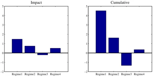
Fig.4 shows the size of the government spending multiplier for each regime. As in Shioji, Takeuchi, and Vu (2010), we compute two types of multipliers. An impact multiplier uses impulse responses for the impact period, and a cumulative multiplier uses the sum of impulse responses for the first 12 quarters. The left panel shows that in Regime 1 only government spending multiplier is substantially larger than one. The impact multipliers are around 70 and 50 percent in Regimes 2 and 4, respectively. As shown in Fig.3, the impact multiplier in Regime 2 is a negative value. In the right panel, the cumulative multiplier is the highest in Regime 1, and we also find that it is larger than one in Regime 2. In Regime 3, the cumulative multiplier becomes much lower than the one at impact.¹⁵

15For a review of the US economy, see, among others, Ramey (2011), who concludes that the multiplier roughly ranges from 0.8 to 1.5.

(10)

Fig.5 shows the response to a one-percent tax shock. The effect of tax shocks on government spending is small and insignificant in most cases. Our prior on output response is that tax increases have a negative effect on output. In Regime 3, however, one distinctive feature is that tax increases significantly expand GDP. Overall, we find that lax fiscal stimuli in Regime 3 rather depressed the macroeconomy.

4.2 Fiscal shocks and business cycles

In this subsection, we assess how important fiscal shocks are in explaining macroeconomic fluctuations. We decompose forecast error variances and historical fluctuations in output into fiscal and non-fiscal components.

4.2.1 Forecast error variance decomposition

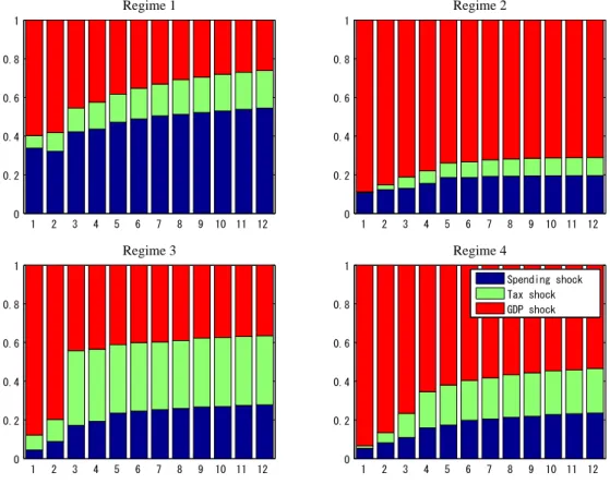
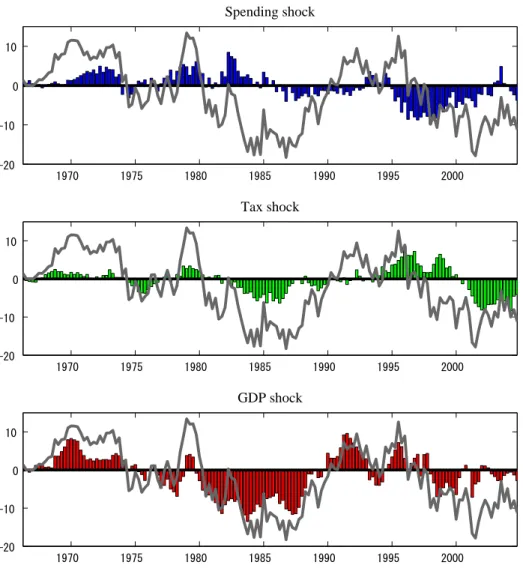
To investigate the relative contribution of fiscal shocks to output fluctuations, we compute the forecast error variance decompositions (FEVD). Fig.6 displays the contributions of each identified structural shocks to the FEVDs of output over a horizon of 12 quarters.

The main findings from the FEVDs are as follows. The relative role of fiscal shocks differs among regimes. In Regime 1, the combination of two fiscal shocks explains roughly 40 percent and 70 percent of the variance of output in the short run and the long run, respectively. In particular, the contribution of the government spending shocks is re- markable. The government spending shock accounts for around 30 percent of the output variance in the short run and 50 percent in the long run. However, in other regimes, the contribution of the government shock becomes minor, explaining roughly 10 percent or less in the short run and roughly 20 percent of the variance after one to three years. In Regime 3, two fiscal shocks contribute 10 to 20 percent of the variance of output in the very short run, and the contribution increases further up to 60 percent. Another distinctive finding is that the tax shock explains a large fraction of output movement in Regime 3. However, the role of the two fiscal shocks becomes minor in Regimes 2 and 4.

Fig.6 is inserted here. 4.2.2 Historical variance decomposition

In this subsection, we perform historical variance decomposition analysis. It is observable that the government spending shocks had a sizable role in increasing output until the mid- 1980s. The negative effect since the mid-1990s is also distinguishable. Tax shocks had a negative effect on output in the 1980s, a positive effect in the mid-1990s, and a negative effect in the 2000s.

Kuttner and Posen (2002) report historical decomposition and show that positive government spending shocks and tax reduction shocks hit the economy in the early 1990s and negative shocks occurred in the late 1990s. The fundamental difference from their results is that positive government spending in Regime 3 has a contractionary effect in our estimated result. Large volumes of stimulus packages were introduced in 1992 and

(11)

1993 after the bubble burst. In our estimation, they have a contractionary effect on output.

5 Effects on consumption and investment

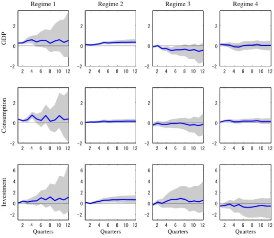
In this and subsequent sections, we examine the response of the components of GDP such as consumption and investment and the external effect on trade balances and the real exchange rate. To understand the effect on each component, we move to a four-variable VAR by including our variable of interest in each estimation. Following Blanchard and Perotti (2002) and Romer and Romer (2010), we order the new variable in last. As before, we include four lags and reestimate the model for each regime.¹⁶

First, we investigate the consumption effects of fiscal shocks. In theory, standard neoclassical models predict a negative effect on consumption,¹⁷ while Keynesian models predict a favorable effect.¹⁸ In Fig.8, we find that positive government spending expands consumption in Regimes 1, 2, and 4. In other words, these findings are more consistent with Keynesian models. However, in Regime 3, we have a significantly negative response of consumption to discretionary government spendings. Negative responses of output and consumption in Regime 3 reconfirm that the large fiscal expansions in the 1990s were inadequate for stimulating the Japanese economy. In response to tax reduction shocks, we also have negative responses of consumption in this regime, while the effects are insignificant in other regimes.

The contractionary effect may reflect that the economy has shifted to the neoclassical economy from the Keynesian economy with the onset of Regime 3. There are several possible stories to explain the contractionary effect on the macroeconomy by an expansionary fiscal policy through low taxes and higher expenditure in Regime 3. One possible explanation is the non-Keynesian effect on the demand side.¹⁹ These studies assert that a fiscal consolidation is sometimes associated with an expansion in private demand. One explanation of this non-Keynesian effect is the concept of “Ricardian Equivalence” by Barro (1974): a tax cut financed by issuing government debt may fail to stimulate private consumption because of future taxation. In other words, fiscal expansion can have contractionary effects on private consumption when households start to believe that such expansion will decrease their lifetime income. Perotti (1999) finds that government expenditure shocks have a positive correlation with private consumption in normal times

16The estimated timings of regime shifts and the results on variance decompositions are almost the same as those in the three-variable benchmark case.

17For example, see Baxter and King (1993) among others.

18The so-called “Keynesian cross diagram” is the basic idea to illustrate the multiplier in a traditional Keynesian model. In the DSGE literature, we need an additional assumption in the typical New Key- nesian models to obtain a high multiplier effect. For example, Gal´ı, L´opez-Salido, and Vall´es (2007) introduce rule-of-thumb consumers and demand-driven employment.

19For reviews of the empirical literature on the non-Keynesian effect in Japan, see Kameda (2009), among others.

(12)

(with low government debt and deficit), but a negative, so-called “non-Keynesian” correlation in bad times. Furthermore, tax shocks have a negative correlation in normal times and a positive correlation in bad times. Regime 3 is the period where the debt-to-GDP ratio skyrocketed from 60 to 100 percent.²⁰ Our conjecture is that households in the early 1990s witnessed low economic growth and a high level of government debt and felt that fiscal expansion was improper to increase their lifetime income.

The second possibility originates from the supply side. As discussed by Caballero, Hoshi, and Kashyap (2008), debt-ridden firms, often referred to as “zombie” firms, prolif- erated during this regime. Based on firm-level regression, they show that the increase in zombie firms depressed the investment and employment growth of non-zombies. Ahearne and Shinada (2005) also find that sectors such as construction and real estate were hard hit by the bubble’s burst in the early 1990s, and that the inefficient zombie firms in these industries prevented more productive companies from entering the market. In turn, public investment during this period was closely related to these industries, and hence expansionary spending may have helped the GDP share of these industries not to be lowered.²¹

Why consumption increases again in Regime 4 is beyond the scope of our research. One possible answer from the existing literature is that the Japanese economy experi- ences the zero lower bound in Regime 4. A growing number of theoretical papers argue that the government spending multiplier can become much larger when monetary policy is constrained by the lower bound of zero on the nominal interest rate. For example, Christiano, Eichenbaum, and Rebelo (2011) find that fiscal policy is considerably effective when the nominal interest rate is zero in a linearized New Keynesian model. Our empirical evidence in this regime can be reconciled with the implications of these theoretical models.

6 Revisiting the twin-deficit hypothesis

The “twin-deficit” hypothesis proposes that fiscal deficits created by cutting taxes or increasing expenditure tend to occur jointly with current account deficits. The traditional Mundell-Fleming model is one of the theoretical models to explain this hypothesis: higher government spending would spur economic activity and, hence, private consumption. Then, the resulting domestic demand would provoke an upward reaction of interest rates that would trigger capital inflows and lead to exchange rate appreciation. As a result, higher final demand and currency appreciation would cause the trade balance to deteriorate.

Most of the empirical studies of the US economy indicate that government deficit shocks cause the trade balance to deteriorate. See, for example, Erceg, Guerri, and Gust (2005) for the US economy, and Ravn et al. (2007) and Monacelli and Perotti (2010) for the US and other three OECD countries. Beetsma et al. (2008) and Castro and Garrote (2012) find similar results for European countries. One exception is Kim and Roubini (2008), who find evidence on the twin convergence hypothesis that government deficit shocks improve the current account.

20For the details of debt dynamics, see Ito et al. (2011).

21In the identification of fiscal shocks, Morita (2012) also uses the relationship between news on fiscal policy and the stock price in the construction sector.

(13)

As for the exchange rates, a number of papers on the US economy, including Corsetti et al. (2009), Kim and Roubini (2008), Monacelli and Perotti (2010), and Ravn et al. (2007) find that the real exchange rate depreciates. In contrast, Beetsma et al. (2008) and Castro and Garrote (2012) find that in the Euro area, higher government spending entails real exchange rate appreciation.

However, there is little empirical evidence for the Japanese economy. Estimating an open-economy DSGE model, Shioji el al. (2010) find that fiscal expansion crowds out exports. Estimating a VAR model with sign restrictions and a DSGE model, Iwata (2012) finds that the trade balance deteriorates on impact, but real exchange rate depreciation induces improvement with some delay.

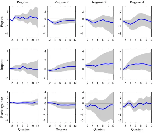
Fig.9 displays the impulse responses of exports, imports, and the real exchange rate to a unit innovation in government spending. First, we find that exports increase but imports decrease in all regimes. In other words, the trade balance deteriorates in response to a government spending shock. This evidence supports that the twin-deficit hypothesis holds in the Japanese economy.²² Second, however, it does not mean that the relationship between the fiscal deficit and the external economy is the same across regimes. If we look at the responses of the real exchange rate, we find that the real exchange rate significantly depreciates in Regime 4, while it appreciates in Regime 1 and is insignificant in Regime 2. Overall, our findings suggest that the evidence on the trade balance and the real exchange rate in Regimes 1 and 2 is in line with the traditional Mundell-Fleming model.

Fig. 9 is inserted here.

7 Concluding remarks

Entering the 1990s, the favorable effect of fiscal policy on output became dubious . How- ever, in the existing empirical works the actual timing of the structural shifts was not fully considered in estimating fiscal shocks. This paper estimates the MS-VAR model of fiscal policy in the Japanese economy to endogenously detect the changes in fiscal policy. We estimate various kinds of models with time-varying and time-invariant coefficients and variances and investigate which model fits the data best.

Three main conclusions can be drawn from our analysis. First, the best-fit model is a version with four regimes that permits both coefficients of independent variables and variances of shocks to vary among regimes. Second, the estimated periods of three regimes are (a) until the mid-1970s, (b) from the mid-1970s to the early 1990s, (c) from the early 1990s to the late 1990s, and (c) from the late 1990s to the end of the sample period. This finding implies that the timing of the structural changes exogenously imposed in the previous literature may be incorrect. Third, the positive estimates of output responses to government spending shocks are generally positive, except for the 1990s, but the sizes and multiplier effects are quite different among regimes. In particular, Regime 2, from the end of the second oil crisis to the end of the bubble period, is the period where the Japanese economy enjoyed the most favorable effect on output of the government shocks. We find a negative effect on output in Regime 3, where lax fiscal policy was insufficient to boost the economy in this period. In Regime 4, we also observe a positive effect on output, but the effect is very short-lived.

22In response to tax shocks, however, we have insignificant results in most cases.

(14)

Extending our benchmark VAR, we also have additional findings. First, positive fiscal shocks expand consumption in Regimes 1, 2, and 4, but decrease consumption in Regime 3. Second, the fiscal effect on output is closely related to the investment. The significantly favorable effect on output in Regime 2 is attributed to the crowd-in of investment, while the insignificant effect in Regime 4 is closely related to the crowd-out of investment. Third, we find that the twin-deficit hypothesis holds in all regimes.

References

[1] Ahearne, A. and N. Shinada (2005): “Zombie firms and economic stagnation in Japan,” International Economics and Economic Policy, 2 (4), pages 363-381.

[2] Barro, R. (1974): “Are government bonds net wealth?” Journal of Political Economy, 82 (6), pages 1095-1117.

[3] Baxter, M. and R. G. King (1993): “Fiscal policy in general equilibrium,” American Economic Review, 83 (3), pages 315-334.

[4] Beetsma, R., M. Giuliodori, and F. Klaassen (2008): “The effects of public shocks on trade balances and budget deficits in the European Union,” Journal of the European Economic Association, 6 (2-3), pages 414-423.

[5] Blanchard, O. and R. Perotti (2002): “An empirical characterization of the dynamic effects of changes in government spending and taxes on output,” Quarterly Journal of Economics, 117 (4), pages 1329-1368.

[6] Caballero, R. J., T. Hoshi, and A. K. Kashyap (2008): “Zombie lending and depressed restructuring in Japan,” American Economic Review, 98 (5), pages 1943-1977. [7] Castro, F. D. and D. Garrote (2012): “The effects of fiscal shocks on the exchange

rate in the EMU and differences with the US,” Banco de Espana Working Papers 1224.

[8] Christiano, L. J., M. Eichenbaum, and S. Rebelo (2011): “When is the government spending multiplier large?” Journal of Political Economy, 119 (1), pages 78-121. [9] Cogley, T. and T. J. Sargent (2005): “Drifts and volatilities: Monetary policies and

outcomes in the post WWII U.S,” Review of Economic Dynamics, 8 (2), pages 262- 302.

[10] Corsetti, G., A. Meier, and G. J. M¨uller (2009): “Fiscal stimulus with spending reversals,” The Review of Economics and Statistics, 94 (4), pages 878-895.

[11] Eguchi, M., (2012): “Zaisei seisakuno koukaha naze sagattanoka? New Keynesian model ni yoru kensyou,” Keio/Kyoto Global COE Discussion Paper (in Japanese). [12] Erceg, C. J., L. Guerrieri and C. Gust (2005): “Expansionary fiscal shocks and the

US trade deficit,” International Finance, 8 (3), pages 363-397.

[13] Fisher, J. D. M. and R. Peters (2010): “Using stock returns to identify government spending shocks,” Economic Journal, 120 (544), pages 414-436.

(15)

[14] Gal´ı, J., D. L´opez-Salido and J. Vall´es (2007): “Understanding the effects of government spending on consumption,” Journal of the European Economic Association, 5 (1), pages 227-270.

[15] Ihori, T., A. Nakazato, and M. Kawade (2003): “Japan’s fiscal policies in the 1990s,” The World Economy, 26 (3), pages 325-338.

[16] Inoue, T. and T. Okimoto (2008): “Were there structural breaks in the effect of Japanese monetary policy? Re-evaluating the policy effects of the lost decade,” Jour- nal of the Japanese and International Economies, 22 (3), pages 320-342.

[17] Ito, A., T. Watanabe, and T. Yabu (2011): “Fiscal policy switching in Japan, the U.S., and the U.K.,” Journal of the Japanese and International Economies, 25, pages 380-413.

[18] Ito, T. and F. S. Mishkin (2006): “Two decades of Japanese monetary policy and the deflation problem,” NBER Chapters, in: Monetary Policy under Very Low Inflation in the Pacific Rim, NBER-EASE, 15, pages 131-202.

[19] Iwata, Y. (2012): “Non-wasteful government spending in an estimated open economy DSGE model: Two fiscal policy puzzles revisited,” ESRI Discussion Paper Series No. 285.

[20] Kameda, K. (2009): “Nihonni okeru hi-Keynese koukano hassei kanousei,” Ihori, T. Fiscal Policy and Social Insurance. Economic and Social Research Institute, Cabinet Office, Government of Japan (in Japanese).

[21] Kameda, K., (2011): “What causes changes in the effects of fiscal policy? A case study of Japan,” mimeo.

[22] Kim, C. J. and C. R. Nelson (1999): “State-space models with regime switching: classical and Gibbs-sampling approaches with applications,” MIT Press Books, edition 1, volume 1, number 0262112388.

[23] Kim, S. and N. Roubini (2008): “Twin deficit or twin divergence? Fiscal policy, current account, and real exchange rate in the U.S.,” Journal of International Economics, 74 (2), pages 362-383.

[24] Ko, J. H. and H. Morita (2011): “Fiscal policy under the debt feedback rule: The case of Japan,” Economics Bulletin, 31 (3), pages 2373-2387.

[25] Ko, J. H. and K. Murase (2012): “The great moderation in the Japanese economy,” Research Center for Price Dynamics Working Paper Series No. 60.

[26] Krolzig, H. M. (1997): “Markov-switching vector autoregressions. Modeling, statistical inference, and application to business cycle analysis,” Springer, Berlin.

[27] Kuttner, K. N. and A. S. Posen (2002), “Fiscal policy effectiveness in Japan,” Journal of the Japanese and International Economies, 16 (4), pages 536-558.

[28] Miyazaki, T. (2010): “The effects of fiscal policy in the 1990s in Japan: VAR analysis with event studies,” Japan and the World Economy, 22 (2), pages 80-87.

(16)

[29] Monacelli, T., and R. Perotti (2010): “Fiscal policy, the real exchange rate and trade goods,” The Economic Journal, 120, pages 437-461.

[30] Morita, H. (2012): “Expansionary effect of an anticipated fiscal policy on consumption in Japan,” Global COE Hi-Stat Discussion Paper Series 219.

[31] Mountford, A. and H. Uhlig (2009): “What are the effects of fiscal policy shocks?” Journal of Applied Econometrics, 24 (6), pages 960-992.

[32] Nakajima, J., M. Kasuya, and T. Watanabe (2011): “Bayesian analysis of time- varying parameter vector autoregressive model for the Japanese economy and monetary policy,” Journal of the Japanese and International Economies, 25 (3), pages 225-245.

[33] Perotti, R. (1999): “Fiscal policy in good times and bad,” Quarterly Journal of Economics, 114 (4), pages 1399-1439.

[34] Ramey, V. A. (2011): “Can government purchases stimulate the economy?” Journal of Economic Literature, 49 (3), pages 673-685.

[35] Ramey, V. A. (2011): “Identifying government spending shocks: It’s all in the timing,” Quarterly Journal of Economics, 126 (1), pages 1-50.

[36] Ravn, M. O., S. Schmitt-Groh´e, and M. Uribe (2007): “Explaining the effects of government spending on consumption and the real exchange rate,” NBER Working Paper Series No. 133228.

[37] Romer, C. D. and D. H. Romer (2010): “The macroeconomic effects of tax changes: Estimates based on a new measure of fiscal shocks,” American Economic Review, 100 (3), pages 763-801.

[38] Shioji, E. (2012): “Time varying effects of public investment and a Stone-Geary production technology,” mimeo.

[39] Shioji, E., T. K. Vu, and H. Takeuchi (2010): “Effects of external and fiscal policy shocks in Japan: Evidence from an open economy DSGE model with partial exchange rate pass-through,” mimeo.

[40] Sims, C. A., and T. Zha (2006): “Were there regime switches in US monetary policy?” American Economic Review, 96, pages 54-81.

[41] Watanabe, T., T. Yabu, and A. Ito (2009): “Estimation of the fiscal multiplier based on institutional information,” Ihori, T. Fiscal Policy and Social Insurance. Economic and Social Research Institute, Cabinet Office, Government of Japan (in Japanese).

(17)

Appendix A Table and Figure

Table 1Log marginal likelihood

Case I

Constant -970.79

Case II Case III Case IV

Variance only Coefficient only All change

2 Regime -929.96 -917.49 -918.63

3 Regime -931.45 -1099.89 -906.38

4 Regime -918.59 -914.49 -901.23

Note: Case I is a time-invariant VAR equation. Case II is an equation with time-varying disturbance variances only. Case III is an equation with time-varying coefficients. Case IV is an equation with

time-varying coefficients and time-varying disturbance variances.

(18)

1970 1975 1980 1985 1990 1995 2000 -0.1

-0.05 0 0.05 0.1

Spending

1970 1975 1980 1985 1990 1995 2000 -0.1

-0.05 0 0.05 0.1

Tax

1970 1975 1980 1985 1990 1995 2000 -0.02

0 0.02 0.04

GDP

1970 1975 1980 1985 1990 1995 2000 -0.06

-0.04 -0.02 0 0.02

Consumption

1970 1975 1980 1985 1990 1995 2000 -0.05

0 0.05 0.1

Investment

1970 1975 1980 1985 1990 1995 2000 -0.1

0 0.1

Export

1970 1975 1980 1985 1990 1995 2000 -0.05

0 0.05 0.1

Import

1970 1975 1980 1985 1990 1995 2000 -0.1

0 0.1

Exchange rate

Fig. 1. Data

Note: All data are transformed in a log-difference form.

(19)

1970 1975 1980 1985 1990 1995 2000 0

0.5 1

Smoothing Probability of Regime 1

1970 1975 1980 1985 1990 1995 2000

0 0.5 1

1970 1975 1980 1985 1990 1995 2000

0 0.5 1

1970 1975 1980 1985 1990 1995 2000

0 0.5 1

Fig. 2. 4-regime all-change smoothing probabilities

(20)

2 4 6 8 10 12 -2

-1 0 1 2 3

Spending

Regime1

2 4 6 8 10 12 -2

-1 0 1 2 3

Regime2

2 4 6 8 10 12 -2

-1 0 1 2 3

Regime3

2 4 6 8 10 12 -2

-1 0 1 2 3

Regime4

2 4 6 8 10 12 -2

0 2

Tax

2 4 6 8 10 12 -2

0 2

2 4 6 8 10 12 -2

0 2

2 4 6 8 10 12 -2

0 2

2 4 6 8 10 12 -1

0 1 2

GDP

Quarters

2 4 6 8 10 12 -1

0 1 2

Quarters

2 4 6 8 10 12 -1

0 1 2

Quarters

2 4 6 8 10 12 -1

0 1 2

Quarters

Fig. 3. Impulse responses to a government spending shock, 4-regime model

Note: Impulses for each regime are given in columns, responding variables in rows. Solid blue and dotted red lines indicate the posterior mean of sampled impulse responses and the 16-th and 84-th

percentile credible intervals, respectively.

(21)

Regime1 Regime2 Regime3 Regime4

−2

−1 0 1 2 3 4 5

Impact

Regime1 Regime2 Regime3 Regime4

−2

−1 0 1 2 3 4 5

Cumulative

Fig. 4. Fiscal multipliers, 4-regime model

Note: The left panel shows the fiscal multipliers of four regimes in the impact period, while the right panel shows the cumulative multipliers for the 12 quarters.

(22)

2 4 6 8 10 12 -1

0 1 2 3

Spending

Regime1

2 4 6 8 10 12 -1

0 1 2 3

Regime2

2 4 6 8 10 12 -1

0 1 2 3

Regime3

2 4 6 8 10 12 -1

0 1 2 3

Regime4

2 4 6 8 10 12 -2

-1 0 1 2 3

Tax

2 4 6 8 10 12 -2

-1 0 1 2 3

2 4 6 8 10 12 -2

-1 0 1 2 3

2 4 6 8 10 12 -2

-1 0 1 2 3

2 4 6 8 10 12 -1.5

-1 -0.5 0 0.5 1

GDP

Quarters

2 4 6 8 10 12 -1.5

-1 -0.5 0 0.5 1

Quarters

2 4 6 8 10 12 -1.5

-1 -0.5 0 0.5 1

Quarters

2 4 6 8 10 12 -1.5

-1 -0.5 0 0.5 1

Quarters

Fig. 5. Impulse responses to a tax shock, 4-regime model

(23)

1 2 3 4 5 6 7 8 9 10 11 12 0

0.2 0.4 0.6 0.8 1

Regime 1

1 2 3 4 5 6 7 8 9 10 11 12

0 0.2 0.4 0.6 0.8 1

Regime 2

1 2 3 4 5 6 7 8 9 10 11 12

0 0.2 0.4 0.6 0.8 1

Regime 3

1 2 3 4 5 6 7 8 9 10 11 12

0 0.2 0.4 0.6 0.8 1

Regime 4

Spending shock Tax shock GDP shock

Fig. 6. Forecast error variance decomposition

(24)

1970 1975 1980 1985 1990 1995 2000 -20

-10 0 10

Spending shock

1970 1975 1980 1985 1990 1995 2000

-20 -10 0 10

Tax shock

1970 1975 1980 1985 1990 1995 2000

-20 -10 0 10

GDP shock

Fig. 7. Historical variance decomposition

(25)

2 4 6 8 10 12 -2

0 2

Regime 1

GDP

2 4 6 8 10 12 -2

0 2

Regime 2

2 4 6 8 10 12 -2

0 2

Regime 3

2 4 6 8 10 12 -2

0 2

Regime 4

2 4 6 8 10 12 -2

0 2

Consumption

2 4 6 8 10 12 -2

0 2

2 4 6 8 10 12 -2

0 2

2 4 6 8 10 12 -2

0 2

2 4 6 8 10 12 -2

0 2 4 6

Investment

Quarters

2 4 6 8 10 12 -2

0 2 4 6

Quarters

2 4 6 8 10 12 -2

0 2 4 6

Quarters

2 4 6 8 10 12 -2

0 2 4 6

Quarters

Fig. 8. Impulse responses to a government spending shock, 4-variable model

(26)

2 4 6 8 10 12 -4

-2 0 2

Regime 1

Exports

2 4 6 8 10 12 -4

-2 0 2

Regime 2

2 4 6 8 10 12 -4

-2 0 2

Regime 3

2 4 6 8 10 12 -4

-2 0 2

Regime 4

2 4 6 8 10 12 -2

0 2 4

Imports

2 4 6 8 10 12 -2

0 2 4

2 4 6 8 10 12 -2

0 2 4

2 4 6 8 10 12 -2

0 2 4

2 4 6 8 10 12 -6

-4 -2 0 2 4

Exchange rate

Quarters

2 4 6 8 10 12 -6

-4 -2 0 2 4

Quarters

2 4 6 8 10 12 -6

-4 -2 0 2 4

Quarters

2 4 6 8 10 12 -6

-4 -2 0 2 4

Quarters

Fig. 9. Impulse responses to a government spending shock, 4-variable model