The 28th Annual Conference of the Japanese Society for Artificial Intelligence, 2014
1D4-OS-11a-3
Size complexity of BDD construction of Pseudo-Boolean constraints
in binary/mixed-radix base form
Naoki Nagatsuka
∗1Masahiko Sakai
∗1Harald Zankl
∗2Keiichiro Kusakari
∗3∗1
Graduate School of Information Science, Nagoya University
∗2
Institute of Compute Science, University of Innsbruck
∗3Faculty of Engineering, Gifu University
An ROBDD with variable order representing a Pseudo-Boolean constraint has polynomial size if all coefficients in the constraint are powers of two (Ab´ıo et al. 2012). This paper extends the result to descending variable-orders and generalizes it to Pseudo-Boolean constraints having mixed-radix base coefficients (for ascending and descending variable-orders). We implemented the proposed constructions and report on experimental results.
1.
Introduction
Pseudo-Boolean (PB) constraints are conjunctions of linear inequalities over Boolean variables. Sev-eral kinds of solvers have been developed, see e.g.
http://www.cril.univ-artois.fr/PB12/ for a compari-son. Typical approaches to solve PB constraints employ Integer Linear Programming (restricted to 0-1 variables), DPLL procedures (regarding PB constraints as generalized clauses [6]), as well as transformations of PB constraints to CNF (via adders, sorting networks, and BDDs [2, 5]).
In [1], Ab´ıo et al. have shown that a PB constraint where all coefficients are powers of two admits a polynomial sized ROBDD with ascending variable-order, i.e., variables hav-ing smaller coefficients are placed closer to the root. Hence, performing a binary expansion of the coefficients in a PB constraint as a pre-processing step yields a polynomial sized ROBDD. For example, a PB constraint 2x+3y≤3 is trans-formed to 2x+ 2y+y′≤3 andy=y′by binary expansion.
In this way, PB constraints can be converted into an equi-satisfiable and polynomial sized CNF via ROBDDs.
Codish et al. proposed the notion of optimal-base de-compositionof a PB constraint, which is a minimal length representation with a mixed-radix base expansion of coeffi-cients [4].
This paper extends the result of [1] to ROBDDs with de-scending variable-order and shows that the ROBDD from a mixed-radix base expanded PB constraint is also of poly-nomial size (for ascending and descending variable-orders). We show experimental results of a MiniSat+ based solver, in which we incorporated the proposed BDD construction.
2.
PB constraints and ROBDDs
A PB constraint is of the forma1x1+· · ·+anxn ≤K,
where the ai’s and K are integers such that ai > 0 and
thexi’s are Boolean variables. Since PB constraints
resem-ble Boolean functions, Binary Decision Diagrams(BDDs) may represent PB constraints. LetCbe the PB constraint
Contact: Naoki Nagatsuka, Nagoya University, C3-1(631) Furo-cho, Chikusa-ku Nagoya, Japan, and [email protected]
x
y
z
1 [30,31]
0
0 1
1
[0,22]
[23,43]
[0,∞)
0 1
(−∞,−1]
0
Figure 1: ROBDD of 9x+ 21y+ 23z≤30
a1x1+· · ·+anxn≤K. We say [β, γ] is theinterval ofC if
forM ∈[β, γ], i.e.,β≤M≤γ,a1x1+· · ·+anxn≤Mand
Care equivalent (seen as Boolean functions) [1]. For a PB constrainta1x1+· · ·+anxn≤K, a variable-order is called
ascendingifxi< xjimpliesai≤ajfor alli, j. Similarly, it
is calleddescendingifxi< xjimpliesai≥aj.
Example 1 A BDD for9x+ 21y+ 23z ≤30with the as-cending orderx < y < zis shown in Figure 1. This is also an ROBDD.
HereROBDDsare a canonical representation for Boolean functions under a given variable order [3]. For an ROBDD, every pair of nodes represents different Boolean functions.
Note that a sub-graph of an ROBDD also is an ROBDD. For example, the node in Figure 1 withselector variabley represents 21y+ 23z ≤M for anyM ∈[23,43]. The fol-lowing propositions state properties used later on where we assume that the ROBDD represents a PB constraint a1x1+· · ·+anxn≤K.
Proposition 2 ([1]) If[β, γ]is the interval of a nodeν in an ROBDD with selector variablexithen:
(i) For each i∈ {1, . . . , n} an assignment {xj = vj}nj=i
exists withaivi+· · ·+anvn=β.
(ii) For each i ∈ {1, . . . , n} an assignment {xj =vj}ij−=11 exists withK−(a1v1+a2v2+· · ·+ai−1vi−1)∈[β, γ].
The 28th Annual Conference of the Japanese Society for Artificial Intelligence, 2014
Proposition 3 ([1]) Letν1andν2be nodes of an ROBDD with the same selector variable. If the intervals of ν1 and ν2 overlap thenν1=ν2.
Proposition 4 Let [β, γ] be the interval of a node of an ROBDD. Thenγ≥ −1.
Proof Suppose γ < −1. Since M ≤ γ < −1 the node is equivalent to the false node, which has the interval
(−∞,−1]. ✷
3.
BDD size of a binary expanded PB
constraint
In [1], Ab´ıo et al. have shown that for a PB constraint where all coefficients are powers of two the ascending order yields a polynomial sized ROBDD. Here we prove that this also holds for the descending order. Note that this result is a special case of Subsection 4.2.
In this section, we consider a PB constraint C of the following form:
(δ0,1·2 0
)x0,1+· · ·+ (δ0,n·2
0 )x0,n
+ (δ1,1·21)x1,1+· · ·+ (δ1,n·2
1 )x1,n
+ · · ·
+ (δm,1·2m)xm,1+· · ·+ (δm,n·2m)xm,n≤K,
where δi,r ∈ {0,1}for alliand r. We consider ROBDDs
with descending order x0,1 > x0,2 >· · · > x0,n > x1,1 >
· · ·> xm,nin this section.
Lemma 5 Let[β, γ]be the interval of a node with selector variablexi,r. Thenβ <(n+r)2i.
Proof Using Proposition 2(i), there must be an assignment to the variables{x0,1, . . . , xi,r}such that
β = (δ0,1·2 0
)x0,1+ (δ0,2·2 0
)x0,2+· · ·+ (δi,r·2i)xi,r
≤ (δ0,12 0
+· · ·+δ0,n2
0 ) +· · ·
+ (δi−1,12i− 1
+· · ·+δi−1,n2i−
1 ) + (δi,12i+· · ·+δi,r2i)
≤ n20
+· · ·+n2i−1 +r2i
.
Here 20 + 21
+· · ·+ 2i−1
= 2i−1. Thus,β < n2i+r2i=
(n+r)2i.
✷
Corollary 6 The number of nodes with selector variable xi,r is bounded by n+r+ 2. In particular, the size of the
ROBDD belongs toO(n2 m).
Proof Letν1, ν2, . . . , νtbe all the nodes with selector
vari-able xi,r. Let [βj, γj] be the interval ofνj. From
Propo-sition 3 we can assume, without loss of generality, that β1 < β2 < · · · < βt. Then −1 ≤ γ1 < β2 < · · · < βt
by Proposition 4. Due to Proposition 2(ii), there is an as-signment such that Kj := K−((δm,n·2m)vm,n+· · ·+
(δi,r+1·2i)vi,r+1)∈[βj, γj]. ClearlyK1< K2 <· · ·< Kt.
Hence Kj+1−Kj ≥2i. Since −1 ≤γ1 < β2 ≤K2 using
Lemma 5, it holds that 0≤K2. Combining βt> Kt−1 > Kt−2+ 2i≥K2+ (t−3)2i≥(t−3)2iwith Lemma 5, we get (n+r)2i> β
t>(t−3)2iand hencen+r+ 2≥t. ✷
4.
BDD size of a mixed-radix base
ex-panded PB constraint
A mixed-radix baseis a sequence⟨b1, . . . , bm⟩of natural
numbers and used as a base coding of a number by a se-quence of small numbers. For example, time and day uses
⟨60,60,24⟩, where the first number represents seconds in a minute, the second one the minutes in an hour, and the last is for the hours in a day. By using this base, 3610 seconds are coded as 10 seconds, 0 minutes, and 1 hour.
Let⟨b1, b2, . . . , bm⟩be a mixed-radix base. We useBifor
the productb1b2· · ·bi for 0 ≤i≤m. Note that B0 = 1.
Using this notation, a sequenceδ0, δ1, . . . , δm, which
satis-fies that 0 ≤ δi < bi+1 for all 0 ≤ i < m, represents a numberδ0B0+δ1B1+· · ·+δmBm.
Example 7 Let ⟨b1, b2, b3, b4⟩ = ⟨3,5,2,2⟩ be a mixed-radix base. ThenB0 = 1, B1 = 3, B2 = 15, B3 = 30, B4 = 60, and 54 is represented as the sequence 0,3,1,1,0 with this base, because0·1 + 3·3 + 1·15 + 1·30 + 0·60 = 54.
Throughout this section, we consider a base⟨b1, . . . , bm⟩
and a PB constraintC′of the following form:
(δ0,1·B0)x0,1+· · ·+ (δ0,n·B0)x0,n
+ (δ1,1·B1)x1,1+· · ·+ (δ1,n·B1)x1,n
+ · · ·
+ (δm,1·Bm)xm,1+· · ·+ (δm,n·Bm)xm,n≤K,
where 0≤δi,r≤bi+1for alliandr. For the simplicity of the proofs, we assume thatδm+1,1=· · ·=δm+1,n= 0 and
bm+1= 1 + max{δm,1, . . . , δm,n}.
4.1 BDD size with an ascending order
In this section we consider an ROBDD of C′ with
as-cending orderx0,1< x0,2<· · ·< x0,n< x1,1<· · ·< xm,n.
We usebmax
for the maximum number ofbi’s, i.e.,bmax =
max{b1, . . . , bm+1}.
Lemma 8 For alli≤m, let[β, γ]be the interval of a node with selector variablexi,r. Then
(i) Bi dividesβ,
(ii) β≤K, and
(iii) K−((r−1)bmax+ (n−r+ 1))B i< γ.
Proof By Proposition 2(i),β can be expressed as a sum of coefficients all of which are multiples ofBi, thusBi
di-videsβ. Proposition 2(ii) gives an assignment to the vari-ables{x0,1, . . . , xi,r}such thatM ∈[β, γ] where
M :=K−((δ0,1·B0)v0,1+· · ·+ (δi,r−1·Bi)vi,r−1). Thusβ≤M≤K−(0 +· · ·+ 0)≤K, and
γ ≥ M
≥ K−((δ0,1B0+· · ·+δ0,nB0) +· · ·
+ (δi−1,1Bi−1+· · ·+δi−1,nBi−1) + (δi,1Bi+· · ·+δi,r−1Bi))
The 28th Annual Conference of the Japanese Society for Artificial Intelligence, 2014
Here δi,j ≤bi+1−1 for anyi, j. We have also (b1−1) + (b2−1)b1+· · ·+ (bi−1)(bi−1· · ·b1) = (bi· · ·b1)−1, i.e.,
(b1−1)B0+ (b2−1)B1+· · ·+ (bi−1)Bi−1< Bi. Thus,
γ ≥ K−(n(b1−1)B0+· · ·+n(bi−1)Bi−1 + (r−1)(bi+1−1)Bi)
> K−(nBi+ (r−1)(bi+1−1)Bi)
= K−((r−1)bi+1+ (n+r−1))Bi
≥ K−((r−1)bmax+ (n+r−1))Bi. ✷
Corollary 9 The number of nodes with a selector variable xi,r is bounded by (r−1)bmax−n+r. In particular, the
size of the ROBDD belongs toO(n2 m).
Proof Let ν1, ν2, . . . , νt be all the nodes with the selector
variablexi,r. Let [βj, γj] be the interval ofνjfor 1≤j≤t.
Since intervals are pairwise disjoint (Proposition 3), we have β1< β2<· · ·< βt. By Lemma 8(i), we getβj−βj−1 ≥Bi
and in particularβ2≤βt−(t−2)Bi. Combining this with
Lemma 8(ii) and (iii), we get K−((r−1)bmax+ (n+r−
1))Bi< γ1≤β2≤βt−(t−2)Bi≤K−(t−2)Bi. Hence
K−((r−1)bmax+ (n+r−1))B
i < K−(t−2)Bi, i.e.,
((r−1)bmax+ (n+r−1))B
i <(t−2)Bi and hence (r−
1)bmax+(n+r−1)> t−2 which gives (r−1)bmax+n+r≥t. ✷
4.2 BDD size with a descending order
In this section we consider an ROBDD ofC′with
descen-ding orderx0,1> x0,2>· · ·> x0,n> x1,1>· · ·> xm,n.
Lemma 10 Let [β, γ]be the interval of a node with a se-lector variablexi,r. Thenβ <(n+r(bmax−1))Bi.
Proof Using Proposition 2(i), there must be an assignment to the variables{x0,1, . . . , xi,r}such that
β = (δ0,1·B0)x0,1+ (δ0,2·B0)x0,2+· · ·+ (δi,r·Bi)xi,r
≤ (δ0,1B0+· · ·+δ0,nB0) +· · ·
+ (δi−1,1Bi−1+· · ·+δi−1,nBi−1) + (δi,1Bi+· · ·+δi,rBi).
Here δi,j ≤ bi+1 −1 for any i, j, and furthermore also (b1−1)B0+ (b2−1)B1+· · ·+ (bi−1)Bi−1< Bi. Thus,
β ≤ n(b1−1)B0+· · ·+n(bi−1)Bi−1+r(bi+1−1)Bi
< nBi+r(bi+1−1)Bi
≤ nBi+r(b
max
−1)Bi. ✷
Corollary 11 The number of nodes with selector variables xi,r is bounded by n+r(bmax−1) + 2. In particular, the
size of the ROBDD belongs toO(n2m).
Proof Letν1, ν2, . . . , νtbe all the nodes with selector
vari-able xi,r. Let [βj, γj] be the interval ofνj. From
Propo-sition 3 we can assume, without loss of generality, that β1 < β2 < · · · < βt. Then −1 ≤ γ1 < β2 < · · · < βt
by Proposition 4. Due to Proposition 2(ii), there is an as-signment such that Kj := K−((δm,n·Bm)vm,n+· · ·+
(δi,r+1·Bi)vi,r+1)∈[βj, γj]. ClearlyK1< K2<· · ·< Kt.
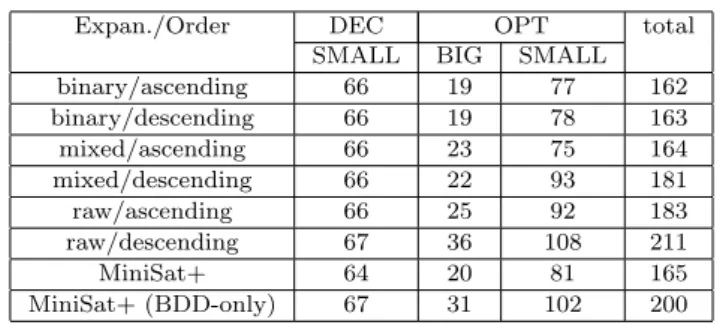
Table 1: Number of solved problems
Expan./Order DEC OPT total
SMALL BIG SMALL
binary/ascending 66 19 77 162
binary/descending 66 19 78 163
mixed/ascending 66 23 75 164
mixed/descending 66 22 93 181
raw/ascending 66 25 92 183
raw/descending 67 36 108 211
MiniSat+ 64 20 81 165
MiniSat+ (BDD-only) 67 31 102 200
HenceKj+1−Kj ≥Bi. Since −1≤γ1 < β2 ≤K2 using
Lemma 10, it holds that 0≤K2. Combiningβt> Kt−1 > Kt−2+Bi ≥K2+ (t−3)Bi≥(t−3)Bi with Lemma 10,
we get (n+r(bmax−1))B
i > βt > (t−3)Bi and hence
n+r(bmax−1) + 2≥t.
✷
5.
Implementation and experiments
We implemented our findings on top of Minisat+ [5] ver-sion 1.0, resulting in the tool GPW. The major extenver-sions are summarized as follows:
• Minisat+ has a function to generate clauses via BDDs constructed from each PB constraint. Thus we at-tached intervals to the nodes of BDDs to reduce re-dundant nodes.
• Binary/mixed-radix base expansion of coefficients be-fore BDD construction. We use the optimal-base [4] as a mixed-radix base for each constraint. Currently, we use the function in Minisat+ for sorting networks that minimizes the sum of digits in the expanded con-straint, where prime numbers up to 17 are allowed for the radices.
We performed experiments on a machine equipped with dual Xeon W5590 (3.33GHz, 4core 8thread, L2cache4*256KB, and L3cache 8MB) processor and 48GB memory. We used MiniSat version 1.14 as underlying solver. The PB benchmarks consist of 306 problems in total; 81, 80, and 145 problems in DEC-SMALLINT-LIN, OPT-BIGINT-LIN, and OPT-SMALLINT-LIN divisions of Pseudo-Boolean Competition 2010, respectively.
Table 1 shows the number of problems that different methods could solve within 600 seconds timeout. The columns correspond to the divisions of problems. The first six rows show the number of problems solved by GPW where we pre-processed the PB constraints to binary or mixed-radix base (first four rows) or did not pre-process (rows five and six). The last two rows show the results for MiniSat+, where the former uses the default strategy and the latter the “BDD-only” strategy.
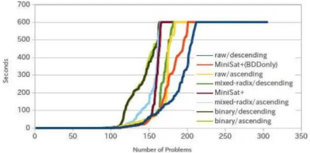
Figure 2 shows the total number of solved problems within the timeout for different methods.
Ignoring divisions of problems, raw/descending (no pre-processing and descending order) scores best. Descending
The 28th Annual Conference of the Japanese Society for Artificial Intelligence, 2014
Figure 2: Runtime for the solved problems
order is better than ascending. Compared with mixed-radix/descending and raw/descending, the former method is faster more than 10 seconds for 17 problems, none of which are BIGINT problems. The latter is faster more than 10 seconds for 61 problems, 17 of which are BIGINT prob-lems. No problems are solved by only the former method, and 29 problems are solved by only the latter method.
All problems solved by binary/descending are also solved by mixed-radix/descending. On the other hand, there are 8 problems solved by binary/ascending but not solved by mixed-radix/ascending.
6.
Concluding remarks
We have shown that the ROBDD for a PB constraint whose coefficients are powers of two has polynomial size, and this also holds in the case that each coefficient is ex-panded by mixed-radix base.
Although the descending order without expansion is es-sentially the same strategy as MiniSat+, the current im-plementation works better than MiniSat+ with BDD-only strategy. Possible reasons of the difference are as follows:
(1) The current implementation construct ROBDD by us-ing intervals introduced by [1]. On the other hand, MiniSat+ can reuse only some of nodes.
(2) The current implementation of intervals requires con-straints to be of the shape a1x1+· · ·+anxn ≤ K.
On the other hand, MiniSat+ constructs a BDD from K′≤a1x1+· · ·+a
nxn≤K.
The current implementation does not allow to mix between non-, binary, or mixed-radix base expansion for each con-straint in a PB problem. Thus, allowing this may improve the performance. We plan to tackle these issues as future work.
Acknowledgments
Supported by the Austrian Science Fund (FWF) project I963 and the Japan Society for the Promotion of Science.
References
[1] Ignasi Ab´ıo, Robert Nieuwenhuis, Albert Oliveras, Enric Rodr´ıguez-Carbonell, and Valentin Mayer-Eichberger. A new look at BDDs for Pseudo-Boolean
constraints. Journal of Artificial Intelligence Research (JAIR), 45:443–480, 2012.
[2] Olivier Bailleux, Yacine Boufkhad, and Olivier Roussel. A translation of Pseudo Boolean constraints to SAT. Journal on Satisfiability, Boolean Modeling and Com-putation (JSAT), 2(1-4):191–200, 2006.
[3] Randal E. Bryant. Graph-based algorithms for boolean function manipulation. IEEE Trans. Comput., 35(8):677–691, August 1986.
[4] Michael Codish, Yoav Fekete, Carsten Fuhs, and Peter Schneider-Kamp. Optimal base encodings for Pseudo-Boolean constraints. In Parosh Aziz Abdulla and K. Rustan M. Leino, editors, TACAS, volume 6605 ofLecture Notes in Computer Science, pages 189–204. Springer, 2011.
[5] N. E´en and N. S¨orensson. Translating Pseudo-Boolean constraints into SAT.Journal on Satisfiability, Boolean Modeling and Computation (JSAT), 2(1–4):1–26, 2006. [6] Christian Herde. Extending DPLL for Pseudo-Boolean constraints. In Efficient Solving of Large Arithmetic Constraint Systems with Complex Boolean Structure, pages 37–58. Vieweg+Teubner, 2011.