Model based Kernel Sum Rule with Applications to State Space Models paper

(1)

Model-based Kernel Sum Rule

with Applications to State Space Models

Yu Nishiyama

The University of Electro-Communications ynishiyam@gmail.com

Motonobu Kanagawa

The Graduate University for Advanced Studies kanagawa@ism.ac.jp

Arthur Gretton University College London arthur.gretton@gmail.com

Kenji Fukumizu

The Institute of Statistical Mathematics fukumizu@ism.ac.jp

Abstract

A model-free Bayesian inference procedure,Kernel Bayes’ rule(KBR), has been proposed for inference in the setting where samples are available from a model, but the model itself may not be available in closed form, or easily computable. The approach has been shown empirically to outperform rejection-based Approximate Bayesian Computation, with greater advantages in high dimensions. In this paper, we develop a novel likelihood-free Bayesian filter for state-space models. The proposed method combines prior knowledge, expressed as state-transition dynam-ics, with a nonparametric observation model learned from data via kernel Bayes’ rule. The resulting inference method applies more generally to hybrid models containing both model-free (learned from data)andmodel-based components. In a robot localization task, the resulting hybrid models outperform both compet-ing inference approaches, and a fully model-free approach which also learns the parametric component.

1 Introduction

A framework for representing probability distributions using positive definite kernels,kernel embed-ding of distributions, has recently been developed in the machine learning community [1]. Briefly, probability distributions are represented as expectations of features in a reproducing kernel Hilbert space (RKHS), where these representations are unique when the RKHS is characteristic [2]. Ap-plications have included nonparametric hypothesis testing [3], feature extraction [4], mapping from distributions to labels [5], and learning of motion models [6]. Conditional distributions may also be represented as RKHS functions [7, 8, 9] (or equivalently, as conditional expectations of the RKHS features), which lead to applications in belief propagation and Bayesian inference [10, 11, 12] and in reinforcement learning [13, 14, 15, 16], where conditional expectations are crucial.

Kernel Bayes’ rule(KBR) [11, 8] is an expression of Bayes’ rule as applied to distribution em-beddings, leading to a likelihood-free (LF) inference method. Specifically, KBR nonparametrically estimates posteriors using training samples(xi, yi)ni=1drawn from a distribution having the desired

(2)

however, KBR does not necessarily require sampling in all its stages, and closed form expressions for the conditional densitiesp(y|x)may be used if available.

The kernel Bayes’ rule may be used as a building block in likelihood-free inference on larger graph-ical models. In this literature, the basic probabilistic operations of the sum rule, chain rule, product rule, and Bayes’ rule are kernelized, and will be denotedkernel sum rule(KSR),kernel chain rule (KCR),kernel product rule(KPR), and KBR, respectively [8]. Combinations of these rules allow kernel Bayesian inference(KBI), i.e. Bayesian inference expressed entirely in terms of distribution embeddings. [7] and [11] proposed filtering algorithms for state space models, using the KSR and KBR, where both the transition dynamics and observation process are learned nonparametrically from training data.

The KBI algorithms described so far have beenfully nonparametric, i.e., all the conditional proba-bilities are learned nonparametrically. In certain applications, however, known probabilistic models might exist, and should be incorporated flexibly within KBI. For example, in state space models of vision-based robot localization [18], the hidden state is a mobile robot’s position, and the observa-tion is an image captured by the robot. The goal is to estimate the robot’s posiobserva-tion using a sequence of images. The mapping from a captured image to information about position is typically complex. By contrast, the transition dynamics of the robot’s position are rather simple, and may be obtained using mathematical models of the physical system, which are encoded as probabilistic models of motion. Thus, it is desirable to combine nonparametric learning of the observation process using KBI, and parametric models of the transition dynamics.

We propose a novel likelihood-free filtering algorithm for state space models, where the observation process is learned by using KBR, and the transition dynamics are modelled explicitly in parametric form, for instance via Gaussian noise models. The results are subset of those given in [19]. We introducemodel-based KSR(Mb-KSR), which is a kernelized sum rule adapted to the case where probabilistic models of conditional distributions are present. We refer to the existing KSR [8] as nonparametric KSR (KSR). We compare two filtering algorithms based respectively on Non-KSR, and the proposed Mb-Non-KSR, on a robot localization task.

2 Preliminaries & Model-based Kernel Sum Rule (Mb-KSR)

See [19, 11, 8] for details. LetP(X)be the set of probability distributions on a measurable space

(X,B(X)). Let(X, k,H)denote the unique reproducing kernel Hilbert spaceHgenerated by a positive definite kernelk:X × X →Ron the setX. Thekernel meanof a probability distribution P ∈ P(X)inHis defined by the mean feature:

mP :=EX∼P[k(·, X)] =

Z

X

k(·, x)dP(x)∈ H.

We also use a notation mX for mP. Ifcharacteristic kernels[2] are used, the kernel mean map

P 7→ mP is guaranteed one to one. In this kernel Bayesian literature,mP is inferred in place of

P. Let(X,B(X))and(Y,B(Y)). Thesum rule is to computeq(y) = R_Xp(y|x)π(x)dxgiven conditional densityp(y|x)and input densityπ(x). Let(X, kX,HX)and(Y, kY,HY). Thekernel

sum rule(KSR) is to compute the kernel mean ofq(y)from the kernel mean ofπ(x). [7, 8] proposed an algorithm for the KSR with nonparametric learning ofp(y|x)from training samples. We refer to it as nonparametric KSR (Non-KSR). Whenp(y|x)is given by certain probabilistic models such as additive Gaussian noise models, we propose to use the model-based KSR (KSR). The Mb-KSR computes the kernel mean ofq(y)by a weighted sum of tractable conditional kernel means of probabilistic models, i.e., the kernel mean ofq(y)is given byPl_i=1γimY|_X˜

ifrom an input kernel

mean estimatorPli=1γikX(·,X˜i)of the densityπ(x). The conditional kernel meanm_Y|_X˜ i has an

explicit form depending on pairs ofp(y|x)and kernelkY. An important difference between the

Non-KSR and Mb-KSR is that the Non-KSR contains a regularization parameter, but the Mb-KSR not - in other words, by using Mb-KSR, we avoid the bias introduced by this regularization. To illustrate: ifp(y|x)is additive Gaussian noise models andkY is a Gaussian kernel, thenm_Y|_X˜

i

(3)

a KBR algorithm with nonparametric learning of p(y|x). Combinations of the KBR, Non-KSR and proposed Mb-KSR yield more flexible kernel Bayesian inference combined with probabilistic models, where the following proposed filtering algorithm is an example.

3 Kernel LF Filtering Algorithms for State Space Models

The setting of state space models to consider here for filtering is as follows:

• Letx∈ X =Rmbe a hidden state. The transition dynamicsp(x′_|_x₎_{comprise an additive}

Gaussian noise modelxt+1 =f(xt) +ςt,ςt ∼N(0,Σ)with a linear/nonlinear function

f :Rm→Rm.

• Letz∈ Z be an observation, whereZis an arbitrary domain such as an Euclidean space, graphs, strings, and images. The observation processp(z|x)is nonparametrically learned from training data{(Xi, Zi)}ni=1assuming likelihood-free.

Letq(xt−1|z1:t−1)denote a belief overX given observationsz1:t−1 := (z1, . . . , zt−1) at time

t−1. Theprediction step (PS) is given by p(xt|z1:t−1) := R

p(xt|xt−1)q(xt−1|z1:t−1)dxt−1.

Thefiltering step(FS) is given byq(xt|z1:t) := p(zt|xt)p(xt|z1:t−1)/ R

Xp(zt|xt)p(xt|z1:t−1)dxt

with a prior p(xt|z1:t−1) and a new observation zt. Let (X, kX,HX) and (Z, kZ,HZ). Let

q(xt|z1:t), respectively. Suppose that we have an estimator for mXt−1|z1:t−1 as mˆXt−1|z1:t−1 =

Pn

i=1[αXt−1|z1:t−1]ikX(·, Xi)with weightsαXt−1|z1:t−1 ∈R

n

and data(X1, . . . , Xn). The kernel

PS is given by the proposed Mb-KSR, as

ˆ

mXt|z1:t−1 =

n

X

i=1

[αXt−1|z1:t−1]imX′|Xi,

wheremX′_|Xi is the conditional kernel mean of the transition dynamics (Gaussian noise model)

given a data pointXi.mX′|Xiis a Gaussian whenkX is a Gaussian kernel. The kernel FS is given

by the KBR [11] with the priormˆXt|z1:t−1 and a new observationzt, as

ˆ

mXt|z1:t=

n

X

i=1

[αXt|z1:t]ikX(·, Xi), αXt|z1:t =RX |Z(βZt|z1:t−1)kZ(zt),

wheren×nmatrixRX |Z(βZt|z1:t−1)depends onβZt|z1:t−1as

RX |Z(βZt|z1:t−1) := D(βZt|z1:t−1)GZ((D(βZt|z1:t−1)GZ) 2

+δnIn)−1D(βZt|z1:t−1),

β_Z_t_|_z

1:t−1 = (GX+nǫnIn)

−1

GX′|XαXt−1|z1:t−1.

HereD(β_Z

t|z1:t−1)is the diagonal matrix of the vectorβZt|z1:t−1.GXandGZ are Gram matrices,

(GX)ij = kX(Xi, Xj)and(GZ)ij = kZ(Zi, Zj), respectively. ǫn andδn are regularization

pa-rameters.GX′|Xis ann×nmatrix given by(GX′|X)ij =mX′|Xj(Xi). As a result, the kernel LF

filtering algorithm is summarized in Algorithm 1.

Robot Localization

We applied the proposed Algorithm 1 to a vision-based robot localization problem. We used the COsy Localization Database (COLD) [18], which contains image sequences captured by mobile robots in indoor laboratory environments. Each imagezis labeled by the robot’s position(x, y, θ)∈

R2_×_[₋_{π, π}_]

(4)

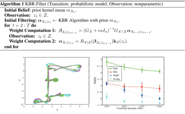
Algorithm 1KBR-Filter (Transition: probabilistic model, Observation: nonparametric) Initial Belief:prior kernel meanmX₁.

Observation: z1∈ Z.

Initial Filtering:αX1|z1 ←KBR Algorithm with priormX1.

for t= 2 :T do

Weight Computation 1: β_Z_t_|_z

1:t−1 = (GX+ǫnIn)

−1

GX′|XαXt−1|z1:t−1.

Observation: zt∈ Z.

Weight Computation 2: αXt|z1:t =RX |Z(βZt|z1:t−1)kZ(zt).

end for

-6 -4 -2 0 2 4 6 8 -10

-8 -6 -4 -2 0 2 4

x y

200 400 600 800 1.5

2 2.5 3 3.5 4 4.5 5

Training Sample Size

R

MSE

NAI NN fKBF Analy

Figure 1: Left; three similar trajectories (colored) of a mobile robot. Each state(x, y, θ)(arrows representθ) is associated with an image. Right; RMSE vs training sample size. Error bars indicate standard deviations.

given the current state(x, y, θ), the current odometry measurement(¯x,y,¯ θ¯), and the next odometry measurement(¯x′,y¯′,θ¯′):

x′ = x+δtranscos(θ+δrot1) +ξx, δrot1= atan2(¯y′−y,¯ x¯′−x¯)−θ,¯

y′ = y+δtranssin(θ+δrot1) +ξy, δtrans= ((¯x′−x¯)

2

+ (¯y′−y¯)2)12,

cosθ′ = cos(θ+δrot1+δrot2) +ξc, δrot2= ¯θ′−θ¯−δrot1,

sinθ′ ₌ _sin(_θ₊_δ

rot1+δrot2) +ξs,

whereξx ∼ N(0, σ2x),ξy ∼ N(0, σy2),ξc ∼ N(0, σc2), andξs ∼ N(0, σs2)are Gaussian noise.

Here,atan2(·,·)is an arctangent function with two arguments. We learned the variancesσ2

x,σ

2

y,

σ2

c, and σs2 using the two training datasets. We used the spatial pyramid matching kernel [21]

for imagesZ and a Gaussian kernel for states(x, y,cosθ,sinθ). The bandwidth parameters and regularization parameters were tuned based on twofold cross-validations using the training datasets. In the test phase, we estimated a filtered state as a training data point that maximized the weight of the posterior kernel mean. We then evaluated the root mean squared error (RMSE) of a test sequence and the result was averaged over10experiments for each training dataset size. We compared the results obtained using the following methods.

Na¨ıve method (NAI): Given a test imagez, the position(x, y, θ)of a robot was estimated as a point in the training dataset that maximized the similarity in terms of the same kernel with spatial pyra-mid matching. Thus, this method did not consider the Markov property of the time series. Nearest Neighbors (NN): Ak nearest neighbor approach is proposed for a nonparametric learning of the observation process [22]. fKBF [11]: this algorithm estimated the hidden states based on non-parametric learning of both the observation process and the transition dynamics. This comparison demonstrated the effect of incorporating knowledge of the odometry motion model.

(5)

References

[1] A. Smola, A. Gretton, L. Song, and B. Sch¨olkopf. A Hilbert space embedding for distributions. InInternational Conference on Algorithmic Learning Theory (ALT), pages 13–31, 2007. [2] B. Sriperumbudur, A. Gretton, K. Fukumizu, G. Lanckriet, and B. Sch¨olkopf. Hilbert Space

Embeddings and Metrics on Probability Measures. Journal of Machine Learning Research, 11:1517–1561, 2010.

[3] A. Gretton, K. M. Borgwardt, M. J. Rasch, B. Sch¨olkopf, and A. J. Smola. A Kernel Two-Sample Test. Journal of Machine Learning Research, 13:723–773, 2012.

[4] K. Fukumizu and C. Leng. Gradient-based kernel method for feature extraction and variable selection. InNIPS, pages 2123–2131. 2012.

[5] K. Muandet, K. Fukumizu, F. Dinuzzo, and B. Sch¨olkopf. Learning from Distributions via Support Measure Machines. InNIPS, pages 10–18. 2012.

[6] L. McCalman, S. O’Callaghan, and F. Ramos. Multi-modal estimation with kernel embeddings for learning motion models. In IEEE International Conference on Robots and Automation (ICRA), 2013.

[7] L. Song, J. Huang, A. Smola, and K. Fukumizu. Hilbert Space Embeddings of Conditional Distributions with Applications to Dynamical Systems. InICML, pages 961–968, 2009. [8] L. Song, K. Fukumizu, and A. Gretton. Kernel embedding of conditional distributions. IEEE

Signal Processing Magazine, 30(4):98–111, 2013.

[9] S. Gr¨unew¨alder, G. Lever, L. Baldassarre, S. Patterson, A. Gretton, and M. Pontil. Conditional mean embeddings as regressors. InICML, pages 1823–1830, 2012.

[10] L. Song, A. Gretton, D. Bickson, Y. Low, and C. Guestrin. Kernel Belief Propagation.Journal of Machine Learning Research - Proceedings Track, 15:707–715, 2011.

[11] K. Fukumizu, L. Song, and A. Gretton. Kernel bayes’ rule: Bayesian inference with positive definite kernels. Journal of Machine Learning Research, pages 3753–3783, 2013.

[12] M. Kanagawa, Y. Nishiyama, A. Gretton, and K. Fukumizu. Monte Carlo Filtering Using Kernel Embedding of Distributions. InProceedings of the Twenty-Eighth AAAI Conference on Artificial Intelligence, pages 1897–1903, 2014.

[13] Y. Nishiyama, A. Boularias, A. Gretton, and K. Fukumizu. Hilbert Space Embeddings of POMDPs. InUAI, pages 644–653, 2012.

[14] S. Gr¨unew¨alder, G. Lever, L. Baldassarre, M. Pontil, and A. Gretton. Modelling transition dynamics in MDPs with RKHS embeddings. InICML, pages 535–542, 2012.

[15] K. Rawlik, M. Toussaint, and S. Vijayakumar. Path Integral Control by Reproducing Kernel Hilbert Space Embedding. Proc. 23rd Int. Joint Conference on Artificial Intelligence (IJCAI), 2013.

[16] B. Boots, G. Gordon, and Arthur Gretton. Hilbert Space Embeddings of Predictive State Representations. InUAI, pages 92–101, 2013.

[17] K. Fukumizu S. Nakagome and S. Mano. Kernel approximate Bayesian computation for population genetic inferences. Statistical Applications in Genetics and Molecular Biology, 12(6):667–678, 2013.

[18] A. Pronobis and B. Caputo. COLD: COsy Localization Database. The International Journal of Robotics Research (IJRR), 28(5):588–594, 2009.

[19] Y. Nishiyama, M. Kanagawa, A. Gretton, and K. Fukumizu. Model-based Kernel Sum Rule. arXiv:1409.5178, 2014.

[20] S. Thrun, W. Burgard, and D. Fox. Probabilistic Robotics. MIT Press, Cambridge, MA, 2005. [21] S. Lazebnik, C. Schmid, and J. Ponce. Beyond bags of features: Spatial pyramid matching for

recognizing natural scene categories. InCVPR, pages 2169–2178, 2006.