Performance of Submillimeter Wavelength
Antenna through the ALMA
Ayumu Matsuzawa
Doctor of Philosophy
Department of Astronomical Science
School of Physical Sciences
SOKENDAI (The Graduate University for
Advanced Studies)
定
Study on the Verification Method of Pointing
Performance of Submillimeter Wavelength Antenna
through the ALMA
Ayumu Matsuzawa
1 / 157
Abstract
The Atacama Large Millimeter/Submillimeter Array (ALMA) is a gigantic radio interferometer array for millimeter to submillimeter wavelengths (10 to 0.3 mm), which is located at Chajnantor Plateau in Chile (an altitude of about 5000 m). The ALMA array includes fifty 12-m antennas (12-m Array), the Atacama Compact Array (ACA; a.k.a., Morita Array), comprising a 7-m antenna array and a total power array with four 12-m antennas. To obtain an observed image with high reliability, all ALMA antennas require high referencing pointing performance, which is the accuracy needed to determine the relative positions of the target star and the reference position (first measured position of the star) during an observation. In ALMA, it is necessary for the referencing pointing performance of the antenna not to exceed 0.6 arcsecs under the primary operating conditions, corresponding to 1/19 and 1/11 of the Half-Power Beam Width (HPBW) of the ALMA 7-m and 12-m antennas, respectively, at the highest observing frequency (950 GHz). All ALMA antennas had been assembled and their scientific and system performances were verified at Operations Support Facility (OSF) of ALMA site (an altitude of about 3000 m) before transporting to high site. This study includes a detailed description of the accuracy verification of various components, including the referencing pointing performance of the ALMA ACA antennas and a physical interpretation of the referencing pointing performance. The referencing pointing performance of an ACA antenna is verified by measurering the Root Mean Square (RMS) of the distance between the centroid positions of the reference positions (the first measured centroid position) and of the target star, in images produced by the Optical Pointing Telescope (OPT) that is mounted in the backup structure of all ACA antennas. It is important to estimate the optical seeing component at the OSF with high accuracy when determining the referencing pointing performance because the optical seeing component accounts for a large portion of the measured value of the referencing pointing measurement. The contribution of optical seeing to the centroid positons of the OPT images is significant when the integration time of the OPT is short, so that in the measurement of the optical seeing with the OPT, an integration time should be one second shorter than that of the referencing pointing measurement (five seconds). In previous research, the time-dependence of the optical seeing was corrected from a Kolmogorov Power Spectrum Density (PSD) [Saito et al. (2012)]. However, it is known that this correction method tends to overestimate the required correction for optical seeing at an integration time of five seconds. In fact, according to earlier studies, the
2 / 157
134 in 458 datasets indicate that the residual between the measured value and the fluctuating components, which randomly change with the measurement date (for example, the optical seeing), becomes negative. These negative residuals may provide to underestimate the referencing pointing performance of the ACA antenna, decreasing the reliability of the verification result for referencing pointing performance. From the PSD, the time-dependence of the optical seeing with some weather parameters (wind velocity, wind attacking angle, ambient temperature, and opacity) had been in detail investigated using multiple regression analysis. From the results of the multiple regression analysis, it was newly found that there is a stronger correlation between a wind velocity and an index of integration time (t), and the relation was finally measured
as − . ± . − . ± . ×�wi when t is an integration time and Vwind is a wind
velocity. On the other hand, in this study, the new relation between the optical seeing and wind velocity, − . , was derived in theory with the Kolmogorov model of turbulence under the observation scale of the OPT is smaller than the outer scale of eddy in the turbulence. When a wind velocity is too small, the measured relation can be represented by − . ± . . This good matching between the theory and measurement results indicates that the new optical seeing correction method was valid for verifying the referencing pointing performance of the ACA antennas. It is therefore proposed in this study that the relation between the power law index and wind velocity is implemented into a new correction method for optical seeing. Using the new correction method, it was confirmed that the negative residuals of 134 in 458 datasets is successfully improved to be 63, suggesting that the new optical seeing correction method is valid for verifying the referencing pointing performance of the ACA antennas. Furthermore, the negative residuals may be caused by uncertainty in determining the reference position (the first measured centroid position). In order to estimate the referencing pointing performance of the ACA, random fluctuation components must be subtracted from the measured pointing results. The reference position will have an effect from the true average of the random fluctuation components. The random fluctuation components for any time is unknown and is not easy to be derived. The uncertainty was assumed in previous research to be comparable to the standard deviation of the random fluctuation components. However, the uncertainty of the reference position may be overestimated under this assumption. In this study, a new estimation method is proposed that uses the average of all measured centroid positions instead of the offset of the reference position. In addition, this method is applied to ACA antennas No. 1 to 4. With new correction method for optical seeing, the number of negative residuals decreases from 24 to 11 in 99 datasets of the four ACA antennas.
3 / 157
Then, with new estimation method of the reference position, the number of negative residuals furthermore decreases from 11 to 2 in 99 datasets. This indicates that most of the negative residuals are resolved by the two new methods that were proposed newly here. In this study, the Az and El dependencies of the optical seeing of the OSF were also verified independently. It was assumed that the optical seeing does not depend on the azimuth (Az) angle; rather, it depends only on the elevation (El) angle as sin (El)-0.5 is derived from the Kolmogorov model of turbulence. Verification tests confirmed that the optical seeing of the OSF does not depend on the Az angle; instead, it depends on the El angle, with the dependence derived from the Kolmogorov model of turbulence. The OPT cannot verify a component that changes on a shorter time scale than the integration time of the OPT (five seconds). In this study, the key component on such a short time scale was also verified by measuring the servo error. The servo error is caused by the antenna servo system that controls the antenna. It was measured by the difference between the readout angle measured by the angular resolver connected to the antenna control unit (ACU) and the angle commanded by the antenna bus master. In order to investigate the contribution of the RMS of servo errors to the referencing pointing performance, the servo errors were measured at various rotational velocities on the azimuth (Az) and elevation (El) axes, ranging the azimuth from 2 to 0.000002 deg/s and an the elevation from 0.2 to 0.000002 deg/s for 210 seconds. Verification tests confirmed that the RMS of servo errors is less than 0.1 arcsecs and enough small to contribute the RMS of servo errors to the referencing pointing performance (0.6 arcsecs). Also of importance, the ALMA antenna must stabilize more quickly to shorten the dead time after fast switching, to enable the observation of a target source and calibrator source to be as near to simultaneously as possible. In this study, the pointing performance during the settling time after fast switching was further verified. Verification tests with the ACA 7-m antenna No. 12 confirmed that the pointing performance during the settling time after fast switching meets the technical specification of the ALMA without directional biases. In conclusion, the referencing pointing performance of the ACA antenna was verified to have higher reliability than that shown in earlier studies.
4 / 157 Index
1 Introduction ... 6
2 Measurement of Referencing Pointing Performance ... 11
3 Development of New Correction Method for Optical Seeing in Referencing Pointing Performance... 23
3.1 Time-Dependence of Optical Seeing with Kolmogorov PSD ... 26
3.2 Relating Optical Seeing to Environmental Parameters ... 31
3.3 Time-Dependence of Optical Seeing and Wind Velocity ... 49
4 Investigations of Servo Error in Referencing Pointing Performance ... 53
4.1 Measurement Methods for investigating Servo Error ... 57
4.2 Measurement Results for investigating Servo Error... 59
4.3 Characteristics of Servo Error at Low Rotation Velocities ... 64
5 Az and El Effects on Optical Seeing due to Atmospheric Path Length ... 68
5.1 Measurement Method for Optical Seeing related to Atmospheric Path Length ... 70
5.2 El Dependence of Optical Seeing on Atmospheric Path Length ... 72
5.3 Az Dependence of Optical Seeing due to Atmospheric Path Length ... 74
6 Pointing Performance during Settling Time after Fast Switching... 80
6.1 Measuring Pointing Performance during Settling Time after Fast Switching ... 81
6.2 Measurement of Pointing Performance during Settling Time after Fast Switching ... 83
6.3 Directional Dependence of Pointing Performance during Settling Time after Fast Switching ... 85
5 / 157
7 Referencing Pointing Performance of ALMA ACA antennas in This Study .... 88
7.1 Referencing Pointing Performance of ACA antennas with New Correction Method of Optical Seeing ... 89
7.2 Validation of New Correction Method of Optical Seeing ... 106
7.3 Physical Interpretation of New Relation between Optical Seeing and Wind Velocity ... 116
8 Conclusion ... 121
8.1 Conclusion and Summary ... 121
8.2 Future Works ... 125
8.3 Suggestions ... 126
Acknowledgments ... 127
References... 129
Appendix A Difference between Size and RMS of Centroid Motion of Star in Distorted Image by Optical Seeing... 132
Appendix B Example of Readout Data of Angles and Rotational Velocities of ACA Antenna... 137
Appendix C Optical Pointing Telescope ... 139
Appendix D Anemometer and Thermometer ... 142
Appendix E Estimation of Centroid Position of Star in Image obtained with Optical Pointing Telescope ... 143
Appendix F Performance of Optical Pointing Telescope ... 147
Appendix G Derivation Method of Optical Seeing Component in Measured Pointing Value ... 148
Appendix H Characteristic of Stars in Measurement of Referencing Pointing .... 157
6 / 157
1 Introduction
Atacama Large Millimeter/Submillimeter Array (ALMA) is a gigantic radio interferometer array operated at Array Operation Site (AOS) (an altitude of 5000 m) on the Chajnantor plateau in northern Chile [1]. The ALMA is a synthesis telescope and consists of 66 antennas; fifty-four 12-m antennas and twelve 7-m antennas [2]. To obtain an astronomical image with high reliability, the ALMA has the array composed of fifty 12-m antenna (12-m Array) and the Atacama Compact Array (ACA, a.k.a. Morita Array) which are composed of the 7-m antennas array and the total power array with four 12-m antennas (Figure 1-2) [3]. All ALMA antennas were assembled and verified at Operations Support Facility (OSF) (an altitude of 2900 m) because hard works at AOS are danger and inefficient for people. The ALMA covers the observations of a millimeter to submillimeter wavelengths (10 to 0.3 mm) and achieves high angular resolution of 0.01 arc-second (hereinafter arcsec) and high sensitivity of 10 micro-Jy in 1 hour at 1mm wavelength in the continuous radiation observation [4].
The output power of an antenna has a gain loss due to the pointing error given by the angular deviation of the peaks of the antenna response from the actual target locations [5]. The requirement of the pointing error depends on the half-power beam width (HPBW) of the antenna. The output power of the antenna has a gain loss of only 0.7% when the pointing error is 1/20 of the HPBW of the antenna assuming that the antenna reception pattern is Gaussian [6]. If a pointing error is large, the output power of the antenna has a large gain loss (e.g. gain loss is 50% when 1/2 of HPBW), and, the image fidelity is declined by an increase of the pointing error. Tsutsumi et al. (2004) have reported the simulation results of the ALMA ACA 7-m antenna observations at 230GHz and 850GHz for various types of radio sources with a pointing error of 0.6 and 1.2 arcsecs [7]. The pointing errors of 0.6 and 1.2 arcsecs correspond respectively to about 1/19 and 1/11 of the HPBW of the ACA 7-m antenna at 950 GHz. According to Tsutsumi et al. (2004), the image fidelity of the ACA 7-m antenna with a pointing error of 0.6 arcsecs is twice that with a pointing error of 1.2 arcsecs in the best case.
In actual radio observations, the antenna switches between a target and a nearby pointing reference, with respect to which the pointing error is measured and corrected with the five-point method (see Section 2). After correcting the pointing error, the antenna switches back to the target source and begins tracking it. This observation process requires the following two conditions:
7 / 157
i) To carry out the five-point method, the pointing reference must come into the field of view (FOV) of the antenna after switching from any direction, and across any angular distance in all sky. This performance is called the absolute pointing performance. The ALMA requires that the absolute pointing error of the antenna shall not exceed 2.0 arcsecs across all sky under the primary operating conditions, a value that is the root sum square (RSS) of average values and standard deviations of the measurement results of the absolute pointing. 2.0 arcsecs is one-third of the FOV of the 12-m antenna at the highest observing frequency (950 GHz). If the absolute pointing performance is within an RSS of 2.0 arcsecs (1σ) after switching from any direction and any angular distance, the star will enter the FOV with a probability of 99.7% (3σ).
ii) To improve the quality of the observed image, the antenna must track the target source and calibration source without a significant pointing error due to the reference source position during the observation. This performance is called the referencing pointing performance (see Figure 1-3). In general, the referencing pointing performance is required to be within 1/20 of the HPBW of the antenna, as mentioned above. In ALMA, it is required that the referencing pointing performance of the antenna shall not exceed 0.6 arcsecs under the primary operating conditions (Table 1-1) [2], [3], [8]. At the highest observing frequency (950GHz), this corresponds to 1/20 and 1/10 of the HPBW of the ALMA 7-m and 12-m antennas, respectively. Although the output power of the antenna has a gain loss with 2.7% when 1/10 of the HPBW, it is not reasonable to specify pointing performance smaller than 0.6 arcsecs in ALMA 12-m antenna, because pointing jitter of about 0.4 arcsecs exists by water vapor content in the troposphere with anomalous refraction at the AOS even under the best conditions [9].
The pointing performance of the ALMA antenna was measured and verified at OSF. The pointing measurement result includes several factors, such as variability in the troposphere, ionosphere, wind, solar radiation, temperature gradient, etc. In order to derive the actual referencing pointing performance of the ALMA antenna, the undesirable effects (troposphere and ionosphere) must be removed from the referencing pointing measurement.
8 / 157
Figure 1-1 Picture of the ALMA at AOS Credit: Clem & Adri Bacri-Normier (wingsforscience.com)/ESO.
Figure 1-2 Pictures of ACA 12-m antenna (left) and ACA 7-m antenna (right).
9 / 157
Table 1-1 Primary operating conditions of the ALMA [8]
Figure 1-3 Example of the measurement result of the referencing pointing. The fluctuation of relative positions of the star from the reference position on the Azimuth axis in time (left) and in space (right).
Primary Operation Conditions Daytime Nighttime Ambient temperature [°C] -20 to +20 -20 to +20
Altitude [m] 5050 5050
Pressure [hPa] 550 550
Precipitation None None
Wind velocity (average) [m/s] 6.0 9.0
Wind velocity (average + gust) [m/s] 6.4 9.5
Solar flux [W/m2] 1290 None
Temperature change in
ambient air temperature [°C/10 min] 0.6 None
10 / 157
The details of measurement verification and the physical interpretation of the referencing pointing performance of the ACA antennas are presented below. More stringent requirements apply to the pointing performance of a submillimeter antenna than those for centimeter wavelengths, assuming the same aperture size for both wavelengths. In order to achieve high pointing performance, it is essential to design and manufacture a high precision antenna. The verification method also requires high accuracy at every point, including the instrument itself, the measurement method, and the analysis of the variables. In this study, first, the verification method used by Saito et al. (2012) in the previous investigation of the referencing pointing performance of the ACA antenna, is checked. The typical verification method for referencing pointing performance and the verification method for OPT according to Saito et al. (2012) are described in Section 2. In this study, the fluctuation of the troposphere at optical wavelengths (called optical seeing) is an important factor in the referencing pointing measurement. In Saito et al. (2012), the optical seeing included in the referencing pointing measurement is measured with the OPT using an integration time of one second shorter than the measurement (five seconds), and the optical seeing is corrected with the time-dependence via the Kolmogorov power spectrum density (PSD) derived from Ukita et al. (2008). However, the correction method using the time-dependence from Kolmogorov PSD may overestimate the correction of optical seeing using an integration time of five seconds. Section 3 presents an investigation of the relation between the power law index of optical seeing for integration times of 1 to 5 seconds and weather parameters (wind velocity, wind attack angle, ambient temperature, and opacity), and the derivation of a new relation between the optical seeing and the wind velocity. Section 4 presents the verification results for the servo error, which is the portion of the pointing error of the antenna that originates in the antenna control of the ACA antenna. Section 5 describes the verification result of the azimuth dependence and the elevation dependence of the optical seeing due to the atmospheric path length at the OSF. Section 6 describes the verification result of the pointing performance during the settling time after fast switching. Section 7 deals with the verification result of the referencing pointing performance of the ACA antenna, together with the time-dependence of the optical seeing derived from this investigation and the physical interpretation of the new relation between the optical seeing and the wind velocity. Finally, Section 8 summarizes the conclusions reached and the future works planned.
11 / 157
2 Measurement of Referencing Pointing Performance
For a general radio telescope antenna, there are two major pointing measurement methods: the five-point method with the receiver that is used an actual observation and the method with an optical pointing telescope (OPT).
In the five-point method, the five output powers are measured at the position of a star and the additional four positions in the directions of positive and negative of an azimuth (hereinafter Az) and an elevation (hereinafter El) from the star separated by a half of the HPBW of the antenna. In general, a bright point source is observed on the five-point method. Assuming that the antenna reception pattern is Gaussian, the pointing error is estimated by fitting two-dimensional Gaussian to the measured output powers at the five positions [10]. The total time required for estimating the pointing error includes a measuring time and a settling time at each position, and a slew antenna time between the positions, that is typically the minute time scale [11].
The OPT is mounted on the back-up structure of the main reflector of the antenna to be aligned with the radio axis. The OPT obtains images in time series of a star with the Charge Coupled Device (CCD) camera. Since the star in each image is blurred and extended due to a fluctuation of the troposphere, however, the centroid position of the star must be in each image for an Az axis and an El axis respectively to determine the position of the star in the image [11]. The pointing error is estimated by determining the root mean square (RMS) of the measured time-variable positions of the star. A typical timescale of obtaining the image is a few seconds, depending on the CCD camera implemented in the OPT ant an image acquiring system [12]. A typical aperture size of the OPT is about 100 to 300 mm [12], [13], [14].
For the pointing measurements of a radio telescope antenna, the OPT method is utilized to verify the pointing performance because the OPT method has three advantages as compared with the five-point method. First, the spatial resolution of the OPT is better than a single radio telescope antenna [11], [13]. For instance, the special resolution of the 12-m diameter radio telescope antenna is about 6.6 arcsecs in a wavelength of 0.32 mm; while the special resolution of 100 mm diameter OPTS is 1.6 to 2.5 arcsecs in wavelengths of 640 to 1000 nm. Second, there are many stars to detect with OPT as compared with the single radio telescope antenna [11]. Third, the OPT can measure the non-repeatable component such as a pointing jitter due to the troposphere by obtaining images in a few seconds, which is faster than a cycle of the estimation of the pointing error with the time-dependence method [16].
12 / 157
Figure 2-1 The ALMA ACA 7-m antenna and optical pointing telescope. Optical pointing telescope is mounted on buck up structure of the main reflector antenna which position indicates as circle.
13 / 157
It is well known that a measured pointing value made using the OPT includes several undesirable effects of the troposphere and the environmental conditions around the antenna [8]. The first undesirable effect is the pointing jitter due to the troposphere at optical wavelengths. This is called the optical seeing, and is caused by variable refraction due to the random motion of turbulent eddies with different refractive indices, which are mainly caused by differences in temperature, pressure, or moisture content [15], [16]. In general, the optical seeing in optical astronomy is quantified by the full width at half-maximum (FWHM) of a point source (star) whose image is broadened and erratically displaced by the refraction of its light as it passes through the atmosphere. In contrast, optical seeing in this study refers to the RMS of the motion of the centroid of the image of a point source (star) that is distorted and displaced by refracted light passing through the atmosphere (hereinafter RMS of centroid positions). The difference between these size measurements of star images is described in Appendix A. The optical seeing may be influenced mainly by wind turbulence in the surface layer and just above the antenna [15]. The second undesirable effect is pointing jitter due to the deformation or the motion of the antenna due to wind load during OPT data acquisition. The pointing jitter due to wind load should be verified at the maximum wind velocity of the primary operating conditions (see Table 1-1) in order to verify the referencing pointing performance under those conditions. However, the wind velocity and pointing jitter due to wind load vary randomly with time. It is difficult to measure the pointing jitter at the maximum wind velocity. Therefore, the pointing jitter due to wind load in the measurement should be subtracted from the measured pointing values. Incidentally, the measured pointing value may include pointing error due to the OPT (For example, the unrepeatable gravitational deformation and the mechanical flexing and slack of the OPT and the joint between the OPT and the ACA antenna. However, any pointing error due to the OPT is considered to be negligible compared to the optical seeing and the pointing jitter due to wind load in the measurement.
On the other hand, the measured pointing value with the OPT does not include pointing components due to the sub reflector, the thermal metrology system of the main reflector, the environmental condition around the antenna, and the antenna servo system. The first missing component is the pointing error due to the vibration and non-repeatable components of gravitational deformation of the sub reflector of the antenna. The second missing component is the performance of the thermal metrology system that actively corrects the pointing errors due to the deformation of the main reflector by thermal load [17]. As mentioned above, the OPT is mounted on the back-up
14 / 157
structure of the main reflector of the antenna (see Figure 2-1). However, the OPT cannot directly measure the components due to the main and sub reflectors because it does not ray trace of the radio axis of the ALMA antenna perfectly. The third missing component is mainly the jitter due to the deformation of the antenna by wind load at the maximum wind velocity that is defined as one of the primary operating conditions (see Table 1-1 in the ALMA). As mentioned above, since the wind velocity and pointing jitter due to wind load change randomly with the date of the measurements, the pointing jitter due to wind load at AOS (9.5 m/s) should be estimated from an finite element analysis by the antenna vendor. The fourth missing component is the inherent error in the antenna servo system that controls the antenna in order to equalize the measured angle and the commanded angle. This is called servo error [18]. The servo error is the measured difference between an input value and an output value, determined by the angle measuring instrument. The servo error includes high-frequency pointing errors due to antenna vibration, etc. on a short time scale of 0.1 seconds, which are smoothed out over the integration time of the OPT.
In order to derive and verify the referencing pointing performance of the antenna, the undesirable components due to the optical seeing and wind load at the average wind velocity during OPT data acquisition must be estimated and removed from the measured pointing value with the OPT. Also, the components due to sub reflector, the main reflector metrology system, the wind load at the maximum wind velocity under primary operating conditions and the servo error must all be estimated and added in the measurement result [8].
The verification method of the referencing pointing performance of the ALMA ACA antenna from Saito et al. (2012) is described. The parameters of the referencing pointing in Saito et al. (2012) are summarized in Table 2-1. The work flow of the verification of the referencing pointing performance in Saito et al. (2012) is shown in Figure 2-2. The measurement of the referencing pointing performance reproduces a typical observation of the ALMA. In the measurement, three to five stars within 4 degrees on the sky are selected, and the antenna switches between these stars every 15 seconds during 900 seconds (Figure 2-3) [8]. The OPT can obtain an image with the integration time of five seconds in the cycle of 15 seconds to achieve a high signal-to-noise ratio. The measured pointing value with the OPT is estimated by the RMS of all relative positions between the reference position (the first measured centroid position) and the centroid positions of the star in 60 images with the integration time of five seconds during 900 seconds (see Figure 2-4). While the referencing pointing performance is measured with the OPT, the weather parameters are obtained with an
15 / 157 anemometer and a thermometer.
The measured pointing value include the pointing error due to the ACA antenna such as the systematic component due to a tracking during 900 seconds, the pointing error due to optical seeing, and pointing jitter due to wind load at the OSF. In Saito et al. (2012), the referencing pointing performance (dθmain) is, from workflow shown in Figure 2-2, represented by
� i = [ � – × � – × � �� + � ��� + �
+ � + � ], (2-1)
where dθ0 is the measured pointing value from the OPT, dθs is the pointing error due to optical seeing, dθtw (OSF) is the pointing jitter due to wind load at the OSF, dθtw (AOS) is the pointing jitter due to wind load at the AOS, dθmr is the pointing error due to the main reflector thermal metrology system, dθsr is the pointing error due to the sub reflector, and dθse is the RMS of servo error. The pointing jitter due to wind load at the AOS, the pointing error due to the main reflector thermal metrology system, and the pointing error due to the sub reflector are estimated from the simulation by the antenna vendor. The fluctuating component, which changes randomly day by day [dθs and dθtw
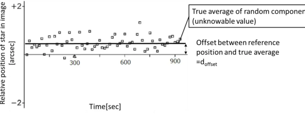
(OSF)] (hereinafter random fluctuating components), must be subtracted twice from the measured pointing value. The measured pointing value from the OPT is estimated by the RMS of deviations of all observed relative positions from the reference position (the first measured centroid position) in both Az and El axes. The reference position has an offset from the true average value of the random fluctuating components, and this offset must be subtracted from the measured pointing value (see Figure 2-5). However, this true average value is an unknowable value. Saito et al. (2012) adopt the standard deviation of the random fluctuating components [dθs and dθtw (OSF)] for the offset between the reference position and the true average value. Consequently, the random fluctuating components must be subtracted twice from the measured pointing value.
The pointing jitter due to wind load at the OSF is estimated by using the ratio of wind force at the AOS and the OSF as follows [19].
� �� = � ��� × [� � /� ��� ] /[P AOS /P OSF ] (2-2)
where V (measure) is the average wind velocity during the measurement of the pointing performance at the OSF, V(AOS) is the maximum wind velocity, 9.5 m/s, for nighttime
16 / 157
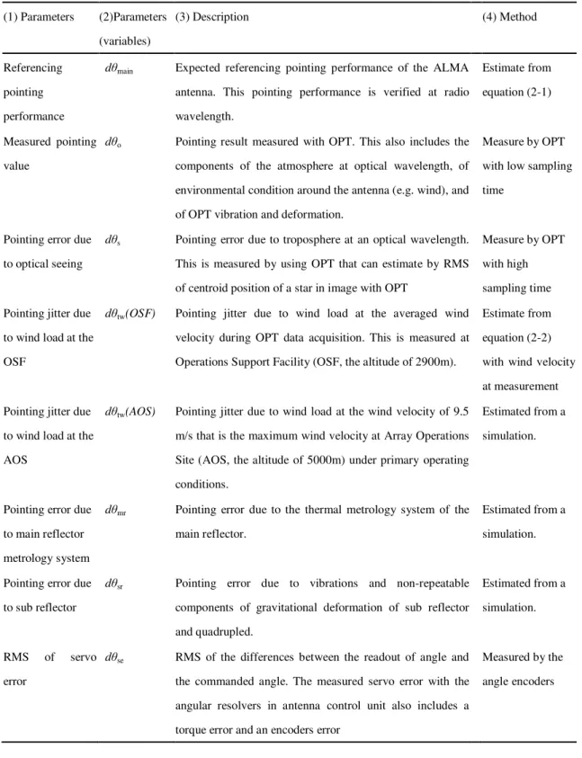
Table 2-1 Summary of parameters of pointing performance of the ALMA ACA antenna
(1) Parameters (2)Parameters (variables)
(3) Description (4) Method
Referencing pointing performance
dθmain Expected referencing pointing performance of the ALMA antenna. This pointing performance is verified at radio wavelength.
Estimate from equation (2-1)
Measured pointing value
dθo Pointing result measured with OPT. This also includes the components of the atmosphere at optical wavelength, of environmental condition around the antenna (e.g. wind), and of OPT vibration and deformation.
Measure by OPT with low sampling time
Pointing error due to optical seeing
dθs Pointing error due to troposphere at an optical wavelength. This is measured by using OPT that can estimate by RMS of centroid position of a star in image with OPT
Measure by OPT with high sampling time Pointing jitter due
to wind load at the OSF
dθtw(OSF) Pointing jitter due to wind load at the averaged wind velocity during OPT data acquisition. This is measured at Operations Support Facility (OSF, the altitude of 2900m).
Estimate from equation (2-2) with wind velocity at measurement Pointing jitter due
to wind load at the AOS
dθtw(AOS) Pointing jitter due to wind load at the wind velocity of 9.5 m/s that is the maximum wind velocity at Array Operations Site (AOS, the altitude of 5000m) under primary operating conditions.
Estimated from a simulation.
Pointing error due to main reflector metrology system
dθmr Pointing error due to the thermal metrology system of the main reflector.
Estimated from a simulation.
Pointing error due to sub reflector
dθsr Pointing error due to vibrations and non-repeatable components of gravitational deformation of sub reflector and quadrupled.
Estimated from a simulation.
RMS of servo error
dθse RMS of the differences between the readout of angle and the commanded angle. The measured servo error with the angular resolvers in antenna control unit also includes a torque error and an encoders error
Measured by the angle encoders
17 / 157
Figure 2-2 Work flow of verification of the referencing pointing performance.
Figure 2-3 Observing stars of the measurement of the referencing pointing performance.
18 / 157
(a) The relative centroid positions of a star in image in Az axis.
(b) Then relative centroid positions of a star in the image on El axis.
Figure 2-4 Example of the referencing pointing measurement which is RMS of centroid positions of a star in the image.
19 / 157
Figure 2-5 Offset between reference position (the first measured centroid position) and a true average of random fluctuating components.
20 / 157
Table 2-2 Difference between the two measurements of the referencing pointing performance and the optical seeing
Referencing pointing performance
Optical seeing
The number of stars 3 - 5 1
The integration time of the OPT 5 [sec] 1 [sec]
The time to determinate the RMS of centroid
positions of a star in image with OPT 900 [sec] 10 [sec]
The number of RMS to measure the result 1 12
under the primary operating condition at the AOS (see Table 1-1), and P (AOS)/ P(OSF) = 0.75 is the atmospheric pressure ratio at the AOS to the OSF.
In Saito et al. (2012), the optical seeing is measured using the OPT before/after the measurement of the referencing pointing performance (see Figure 2-6). To measure the optical seeing, the OPT takes 120 images with an integration time of one second while tracking a star for 120 seconds, and the 120 images are divided into 10-second groups. The RMS of centroid positions is estimated from the ten images obtained in each 10-second interval. The optical seeing is then estimated from the average of the twelve RMSs of centroid positions (see Figure 2-6). The measurement of optical seeing differs from that of the referencing pointing in the following three ways: i) the integration time of the measurement of optical seeing (one second) is shorter than the measurement for the referencing pointing (five seconds), to increase the contribution of the optical seeing. The difference in the integration times of the two measurements is corrected using the time-dependence of the optical seeing from Kolmogorov power spectrum density (PSD) according to Ukita et al. (2008). The verification of this correction method in this study is described in Section 3. ii) The direction of the star between two measurements is different. The measurements of the referencing pointing are performed towards the differing directions at each measurement to verify performance in various directions across the entire sky. In contrast, the optical seeing measurement is performed using pre-selected stars. Since the integration time of the optical seeing is 1/5 that of the measurement for referencing pointing, the star used in the optical seeing is √5 times (star of magnitude +1) brighter than the star used in the referencing pointing. Therefore, the direction of the star between two measurements is often different by several tens of degrees. The optical seeing contributions between the two different directions are different because the optical seeing is related to the atmospheric path length. The difference in direction between the two measurements is corrected by the Az and El dependence of the optical seeing due to the atmospheric path
21 / 157
length. The verification of this correction method in this study is described in Section 5. iii) The RMS of centroid positions is calculated from the centroid position of images obtained within 10 seconds of each other to avoid the effect of pointing error due to lengthy tracking. These differences between two measurements are listed in Table 2-2.
The RMS of servo error is measured as the RMS of time-variable differences between readout angles measured by the angular resolver connected to the antenna control unit (ACU) and the angles commanded by the antenna bus master (see Appendix B) [21]. The ACU outputs the angles every 0.048 seconds. However, the angle measured with the angular resolver is affected by the antenna control, and the servo error includes a torque error due to incomplete suppression of external disturbances and detection error in the angle resolvers and resolvers-to-digital converter, in addition to error due to the antenna control by the ACU. If the instruments of the ACA antenna and the antenna control by the ACU have a problem, the servo error of the angular resolver may become large. Therefore, to check the ACU by measuring the servo error is important. The investigation of the servo error in this study is described in Section 4.
22 / 157
Figure 2-6 Typical measurement process of the referencing pointing and the optical seeing in Saito et al. (2012). The nearest optical seeing measurement result is referred to verify the referencing pointing performance.
23 / 157
As described in Section 2, the measured pointing value includes the referencing pointing performance of the ACA antenna, the pointing error due to optical seeing conditions (hereinafter: optical seeing), and the pointing jitter due to wind load during measurement at the OSF. In order to estimate the referencing pointing performance of the ACA antenna, the optical seeing and the pointing jitter due to wind load must be properly subtracted from the measured pointing value. Since the optical seeing accounts for a large portion of the measured pointing value, it is important to estimate the components of the optical seeing with high accuracy. Note that this optical seeing is different from the full width at half-maximum (FWHM) of a star image. In general, the optical seeing at the telescope site is investigated by a differential image motion monitor (DIMM) set at ground level [24], [25]. However, the DIMM set at ground level cannot measure the optical seeing at the height of the antenna (about 10 m above ground level). Moreover, the DIMM cannot measure low-frequency fluctuations (fluctuations on a scale larger than the aperture size), and may underestimate the optical seeing compared to a single aperture OPT [24]. Therefore, the single aperture OPT mounted on the ACA antenna is more appropriate for estimating the optical pointing components included in the measured pointing value.
The integration time of the referencing pointing measurement is longer than the optical seeing measurement to reduce the contribution of the optical seeing and as a result, the referencing pointing performance of the ACA antenna becomes more dominant. Therefore, the integration time is five seconds (with a sampling rate of 0.2 Hz) typically for the measurement of the referencing pointing [8]. On the other hand, for measuring the optical seeing, a short integration time of one second is more reasonable, to increase the contribution of the optical seeing and to obtain a solely optical seeing component. In Saito et al. (2012), the integration time for the optical seeing measurement was one second [8]. The difference in the integration times of the two measurements is corrected using the time-dependence of the optical seeing (dθs) from Kolmogorov power spectrum density (PSD) according to Ukita et al. (2008) as follows,
� ∝ − . , (3-1)
where t is the integration time. However, in Ukita et al. (2008), the measured optical seeing from an integration time longer than one second indicates a different relationship
24 / 157
with the time-dependence from Kolmogorov PSD [20]. Therefore, the corrected optical seeing with an integration time of five seconds may be overestimated by the correction method for the time-dependence from Kolmogorov PSD (see Figure 3-1) [23]. In Saito et al. (2012), the residuals of the reference pointing measurement after subtracting the optical seeing became negative values for one-third of all the measurement results, which may have been caused by the overestimation of optical seeing. However, the difference between the measured optical seeing and the time-dependence from Kolmogorov PSD for integration times longer than one second has not been investigated.
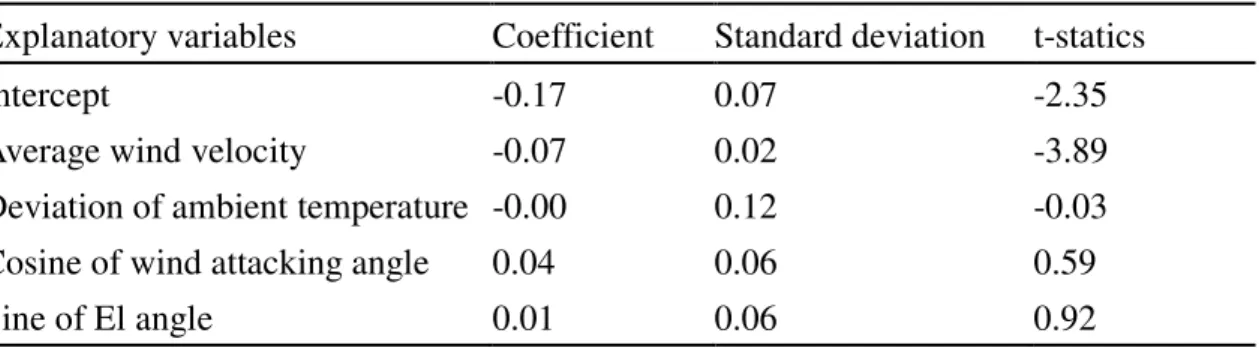
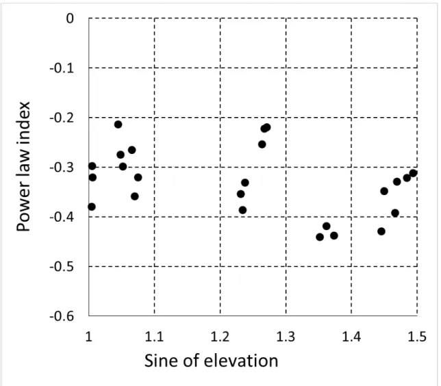
In this study, RMSs of centroid positions with various integration times (1/20, 1/10, 1/5, 1/2, 1, 2, 5, 10, 20, and 50 seconds) were measured in order to investigate the difference between the measured optical seeing (RMS of centroid positions) and the power law relationship from Kolmogorov PSD. The power law index of the RMS of centroid positions with integration times of 1 to 5 seconds was calculated. Optical seeing may be affected by weather conditions, such as wind velocity, wind attack angle, ambient temperature, and opacity. The relationship between the power law index and the quantitatively expressed weather parameters was investigated by multiple regression analysis, which confirmed that the average wind velocity during measurement is strongly correlated with the power law index. In contrast, the scatter of the corrected power law indices with the wind velocity became small, indicating that only the average wind velocity determines the power law indices, so they can be well corrected using the average wind velocity. Finally, a new correction method for optical seeing, including the wind velocity, was derived in this study.
The derivation of the time-dependence from Kolmogorov PSD is described in Section 3.1. The result of multiple regression analysis between the power law indices as criterion variables and the four weather parameters as explanatory variables and the derivation of the new relation between the power law index and wind velocity are described in Section 3.2. The relation between the corrected power law index and the wind velocity and the four weather parameters (the wind velocity, the wind attacking angle, an ambient temperature, and opacity), and the derivation of the new correction method of the optical seeing are described in Section 3.3.
25 / 157
Figure 3-1 Conceptual diagram of the overestimation of the optical seeing at the integration time of five seconds with the correction by the time-dependence according to Ukita et al. (2008).
26 / 157
3.1 Time-Dependence of Optical Seeing with Kolmogorov PSD
Ukita et al. (2004) first provided the relation of the time-dependence of optical seeing from a Kolmogorov power spectrum density (PSD) but did not derive it in theory. In this section, the time-dependence of optical seeing with the Kolmogorov model of turbulence is derived in theory.
Atmospheric turbulence is well described with Kolmogorov model of turbulence, which shows the turbulence of incompressible fluids. Since the Reynolds number of the atmosphere is large (about 107 to 108), the atmosphere is considered to be turbulent [26] under the condition caused when a wind shear generates an eddy between two wind currents of different velocities (see Figure 3-2). In the Kolmogorov model of turbulence, the kinetic energy associated with large-scale eddies’ motions is transferred to smaller and smaller size eddies until it is finally dissipated into heat by viscous friction (see Figure 3-3). The size of the smallest eddy generated from an eddy of the outer (largest) scale is called inner scale. Since the Kolmogorov model of turbulence has self-similarity in general, the rate of dissipation from the outer to the inner scale will become constant (see Figure 3-4). From Figure 3-4, the Kolmogorov model of turbulence in energy decreases according to a power law in the progression from the outer to the inner scale (inertial scale) [27]. The phase structure function [Dφ(r)] of the Kolmogorov model of turbulence is
ϕ = . (L > r > l), (3-2)
where r is the scale of eddy in turbulence, L is the outer scale, l is the inner scale, and r0
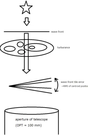
is the Fried parameter [28]. The surface layer that extends to about one km above the ground dominates most of the optical path fluctuation [15]. In addition, the optical seeing may depend mainly on the optical path fluctuations in the surface layer, and some turbulence will occur near the antenna from the direct interaction of wind and antenna. The velocity of such turbulence is represented by the wind velocity at the height of the antenna (or the OPT mounted on the antenna), assuming frozen flow [29]. The RMS of centroid positions in the OPT images is given approximately by the RMS of the wave-front tilt error in observation scale of the telescope (dobs) (Figure 3-5). Assuming that the path fluctuations on the near field, the observing scale of the telescope can correspond to the aperture size of the telescope dapeture (dobs= dapeture). The RMS wave-front tilt error (σ) in the observation scale of the telescope is represented by
27 / 157 (see Appendix A) [24],
� ≅ ��[ ϕ ] ∝ − , (3-3)
where λ is the wavelength.
A consideration of the wave-front tilt in any observation scales is derived as follows. A wave-front tilt along x and y directions are defined as
, ≡ �� , = �� �� � , (3-4)
, ≡ �� , = �� �� � , (3-5)
where l(x,y) is the optical path length, φ(x, y) is the phase of optical wave (see Appendix A). The power spectra of the wave-front title along x and y directions [� ⃗ and
� ⃗ ] are related to the power spectrum of the phase [�ϕ ⃗ ] by
�� ⃗ = �ϕ ⃗ (3-6)
� ⃗ = �ϕ ⃗ (3-7)
where x and y are the components of the spatial frequency . The variance of the wave-front tilt along say x direction is
� = ∫ �ϕ ⃗ ⃗, (3-8)
and the total variance of x and y direction is
� = ∫| | �ϕ ⃗ ⃗, (3-9)
A rigorous analysis of this problem was carried out by Fried, D. L (1965) [15], [28], [30] as
� = . − − , (3-10)
� ∝ − . (3-11)
28 / 157
Finally, equation (3-11) shows the same relation with equation (3-3), giving us the relation at any observation scales in the aperture.
Assuming the frozen flow according to Taylor (1938) [29], so that a perturbed wave-front is swept across the aperture, the observation scale (dobs) becomes Vwind
×t+dapeture where Vwind is a wind velocity and t is an integration time. When Vwind ×t is
larger than dapeture or dapeture is smaller than the outer scale, the observation scale is only dominated by the product of the wind velocity and the integration time, dobs = Vwind× t. Thus, the RMS wave-front tilt error (σ) is represented by
� ≅ ��[ ϕ��wi × ]
wi × ∝ � i
− ∙ − ∝ − . …… ∝ − . . (3-12)
The optical seeing (dθs) corresponds to the RMS wave-front tilt error (σ). The newly estimated index of the time-dependence of optical seeing, -0.17, is a little bit smaller than an amount of -0.2 that was empirically proposed in Ukita et al. (2004) [see equation (3-1)]. In this study, the time-dependence of optical seeing with Kolmogorov PSD, equation (3-12), is newly derived in theory.
29 / 157
Figure 3-2 Conceptual diagram of eddies in the turbulence. Small eddies occur around large eddies secondary.
Figure 3-3 Conceptual diagram of the energy flow in the inertial scale of the Kolmogorov model of turbulence.
30 / 157
Figure 3-4 Kolmogorov energy spectrum of the Kolmogorov model of turbulence. is the wave number, L0 is the outer scale, and l0 is the inner scale.
Figure 3-5 Conceptual diagram of the generation of the wavefront tilts error in the scale of the observation of the telescope (aperture size is 100 mm).
31 / 157
3.2 Relating Optical Seeing to Environmental Parameters
In this study, the RMSs of centroid positions at various integration times were measured using the OPT mounted on the ALMA ACA 7-m antenna No. 12, to investigate the time-dependence of optical seeing. The specifications of the OPT, the detail of the anemometer and the thermometer, the estimation of the RMS of centroid positions with the OPT, and the quality of the RMS of centroid positions are given in Appendix C, Appendix D, Appendix E, Appendix F, respectively. Results indicate that the measured RMS of centroid positions can be attributed entirely to the optical seeing (see Appendix G).
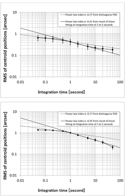
The measurement results of the RMSs of centroid positions with integration times of 1, 2, and 5 seconds and the power law indices from integration times of 1 to 5 seconds with linear fitting are listed in Table 3-1 and Table 3-2. The plots of the RMSs of centroid positions and the results of linear fitting are shown in Figure 3-7, Figure 3-8, Figure 3-9, and Figure 3-10. The dashed line is the time-dependence from Kolmogorov PSD [see equation (3-12)]. The OPT obtains the image with an integration time of 1/30 seconds while tracking the star for 900 seconds. The RMS of centroid positions is measured by the RMS of the centroid positions relative to the reference positions of the star in the image with an integration time of 1/30 seconds. The reference positions are determined by the average of centroid positions within one second from the start time of the measurement (see Figure 3-6). The RMSs of centroid positions with integration times of 1/20, 1/10, 1/5, 1/2, 1, 2, 5, 10, 20, and 50 seconds are measured by the RMS of the integrated relative centroid positions. From these Figures, RMSs of centroid positions with integration times longer than one second indicate a different time-dependence from Kolmogorov PSD, which is similar to the tendency reported in Ukita et al. (2008).
The power law indices are estimated by the RMSs of positions of the star in images with integration times of 1, 2, and 5 seconds, made every 300 seconds. These images, with an exposure time of 1/30 seconds were obtained by OPT during 900 seconds. However, RMSs are estimated every 300 seconds in order to consider the average wind velocity as well as the wind attack angle, which changes on a short time scale [21]. The power law indices of the RMS of centroid positions with integration times of 1, 2, and 5 seconds may be affected by the weather parameters (wind velocity, wind attack angle, ambient temperature, and opacity). In this study, multiple regression analysis was performed with the power law indices as criterion variables and the four weather parameters as explanatory variables.
32 / 157
Figure 3-6 Example of integrated relative centroid positions with the various integration times and the calculation of RMSs of centroid positions. The relative positions with the integration time of 1/30 seconds are raw data. Other RMSs of centroid positions are obtained by similar calculation.
33 / 157
Table 3-1 Summary of measurement results of RMSs of centroid positions in the integration time of 1, 2, and 5 seconds and power law indices between integration time of 1 to 5 seconds.
(1) Date (2) Start (3) End (4) RMS of centroid positions (5) Power law index
in 1 to 5 seconds
(UT) (UT) Integration time
1 second 2 second 5 second
[hh:mm] [hh:mm] [arcsec] [arcsec] [arcsec]
1st 300 seconds 0.90 0.69 0.44 -0.44
2012/6/11 3:43 3:58 2nd 300 seconds 0.89 0.67 0.45 -0.41
3rd 300 seconds 1.08 0.79 0.54 -0.44
1st 300 seconds 0.34 0.26 0.20 -0.32
2012/6/11 5:06 5:21 2nd 300 seconds 0.30 0.25 0.18 -0.3
3rd 300 seconds 0.41 0.31 0.22 -0.38
1st 300 seconds 0.54 0.43 0.30 -0.35
2012/6/11 5:43 5:58 2nd 300 seconds 0.64 0.52 0.33 -0.39
3rd 300 seconds 0.65 0.54 0.38 -0.33
1st 300 seconds 0.37 0.32 0.27 -0.21
2012/6/15 2:29 2:44 2nd 300 seconds 0.37 0.31 0.24 -0.27
3rd 300 seconds 0.34 0.29 0.21 -0.29
1st 300 seconds 1.06 0.86 0.60 -0.34
2012/6/15 4:05 4:20 2nd 300 seconds 1.09 0.80 0.59 -0.39
3rd 300 seconds 1.06 0.86 0.63 -0.32
1st 300 seconds 0.74 0.64 0.49 -0.25
2012/6/16 2:16 2:31 2nd 300 seconds 0.79 0.68 0.55 -0.22
3rd 300 seconds 0.48 0.41 0.33 -0.22
1st 300 seconds 0.31 0.26 0.20 -0.26
2012/6/16 2:51 3:06 2nd 300 seconds 0.41 0.32 0.23 -0.36
3rd 300 seconds 0.57 0.45 0.35 -0.32
1st 300 seconds 1.04 0.86 0.63 -0.31
2012/6/16 3:33 3:48 2nd 300 seconds 1.01 0.78 0.60 -0.32
3rd 300 seconds 1.02 0.75 0.51 -0.42
Table 3-2 Summary of averages and standard deviations of the RMSs of centroid positions in the integration time of 1, 2, and 5 seconds, and the average of power law index between integration time of 1 to 5 seconds.
(1) Date (2) Start (3) End (4) Average of RMSs of centroid positions
(5) Standard deviation of RMSs of centroid positions
(6) Average of power law indices in 1 to 5 seconds
(UT) (UT) 1 second 2 second 5 second 1 second 2 second 5 second
[hh:mm] [hh:mm] [arcsec] [arcsec] [arcsec] [arcsec] [arcsec] [arcsec]
2012/6/11 3:43 3:58 0.96 0.72 0.47 0.11 0.06 0.05 -0.43
2012/6/11 5:06 5:21 0.35 0.28 0.20 0.06 0.03 0.02 -0.33
2012/6/11 5:43 5:58 0.61 0.49 0.34 0.06 0.06 0.04 -0.36
2012/6/15 2:29 2:44 0.36 0.31 0.24 0.02 0.02 0.03 -0.26
2012/6/15 4:05 4:20 1.07 0.84 0.61 0.02 0.04 0.02 -0.35
2012/6/16 2:16 2:31 0.67 0.58 0.46 0.17 0.14 0.11 -0.23
2012/6/16 2:51 3:06 0.43 0.34 0.26 0.13 0.10 0.07 -0.31
2012/6/16 3:33 3:48 1.02 0.80 0.58 0.02 0.05 0.06 -0.35
34 / 157
Figure 3-7 RMS of centroid positions with integration times taken at UT3:43 - 3:48, June 11, 2012 (upper) and UT5:06 - 5:21, June 11, 2012. The averaged wind velocities are 3.16 m/s (upper) and 2.90 m/s (lower). A dashed line is the time dependencies from Kolmogorov PSD. The solid lien is the result of linear fitting of the RMS of centroid positions in integration time of 1 to 5 seconds [see column (5) in Table 3-2].
35 / 157
Figure 3-8 RMS of centroid positions with integration times taken at UT5:43 - 5:58, June 11, 2012 (upper) and UT2:29 - 2:34, June 15, 2012. The averaged wind velocities are 3.39 m/s (upper) and 1.30 m/s (lower). A dashed line is the time dependencies from Kolmogorov PSD. The solid lien is the result of linear fitting of the RMS of centroid positions in integration time of 1 to 5 seconds [see column (5) in Table 3-2].
36 / 157
Figure 3-9 RMS of centroid positions with integration times taken at UT4:05 - 4:20, June 15, 2012 (upper) and UT2:16 - 2:31, June 16, 2012. The averaged wind velocities are 3.23 m/s (upper) and 1.52 m/s (lower). A dashed line is the time dependencies from Kolmogorov PSD. The solid lien is the result of linear fitting of the RMS of centroid positions in integration time of 1 to 5 seconds [see column (5) in Table 3-2].
37 / 157
Figure 3-10 RMS of centroid positions with integration times taken at UT2:51 - 3:06, June 16, 2012 (upper) and UT3:33 - 3:48, June 16, 2012. The averaged wind velocities are 2.28 m/s (upper) and 3.29 m/s (lower). A dashed line is the time dependencies from Kolmogorov PSD. The solid lien is the result of linear fitting of the RMS of centroid positions in integration time of 1 to 5 seconds [see column (5) in Table 3-2].