平成 30 年度 修 士 論 文
DA変換器の線形性向上および
サボニウス風車の高性能化の研究
指導教員 小林 春夫 教授
桑名 杏奈 助教
群馬大学大学院理工学府 理工学専攻
電子情報・数理教育プログラム
姚 丹
contents
I. Improve Linearity of DA Converter ... 3
1. Introduction ... 3
1.1 Research Background ... 3
1.2 Configuration and Operation of Segment DAC ... 4
2 Circuit Element Characteristics ... 6
2.1 Variations in Circuit Element Characteristics ... 6
2.2 Unary DAC Nonlinearity ... 9
3. Magic Square Layout Technique ... 12
3.1. Features of Magic Square ... 12
3.2. Algorithm Using Concentric Magic Square ... 13
3.3. Analysis Results and Consideration ... 14
3.3.1. Linear Gradient Error ... 14
3.3.2. Quadratic Gradient Error ... 15
3.3.3 Linear and Quadratic Joint Gradient Errors ... 16
4. Latin Square ... 17
4.1 Characteristics of Latin Square ... 17
4.2Latin Square Layout Algorithm ... 17
5. Conclusion ... 24
II. Improve the performance of Two-stage Savonius wind turbines ... 25
1. Introduction ... 25
2. Background and Purpose of Research ... 26
2.1 Horizontal Axis Wind Turbine ... 27
2.2 Vertical Axis Wind Turbine ... 28
2.3 Lift Type and Drag Type Wind Turbine ... 28
2.4 Savonius Wind Turbine ... 29
2.5 Improvement of Savonius Wind turbine ... 31
3. Numerical Solution ... 33
3.1 Calculation Area and Boundary Condition ... 33
3.2 Coordinate System ... 34
3.4 General Coordinate Transformation ... 36
3.5 Fractional Step Method ... 37
3.6 Difference ... 38
3.7 Definition of the shape of the wind turbine ... 40
3.8 Parameters for Wind Turbine Output ... 42
3.9 Calculation of Torque ... 43
4. Results and Considerations ... 45
4.1 Self-starting Characteristics of Wind Turbine ... 45
4.3 Dynamic Characteristics of Wind turbine ... 48
4.4 Flow Field around Wind Turbine ... 49
5. Conclusion and Discussion ... 52
5.1 Conclusion and Discussion... 52
5.2 Future Issues ... 52
References ... 54
I. Improve Linearity of DA Converter ... 54
II. Improve performance of Sabo two-wind turbines... 55
Research Achievements ... 57
I. Improve Linearity of DA Converter
1. Introduction
1.1 Research Background
Because of the demand for small-sized high-speed electronic devices, digital
circuits should be adopted. Along with the progress of digitization, many electronic
devices are equipped with digital-to-analog converters (DACs) [1, 2]. Systematic
relative variations exist in MOSFET characteristics, R, C values and so on,which
are on a silicon wafer constituting a semiconductor device. Because characteristics,
values have a slope depending on layout. Due to these reasons above,there is a
problem of linearity degradation of DAC input/output characteristics.
In this paper we have presented a layout algorithm, which is based on magic square
and Latin square properties, to cancel the systematic mismatches among unit cells and
improve the DAC overall linearity. Magic and Latin squares have been investigated
from long time ago by many mathematicians, and there are a lot of theoretical
research results. However, according to our knowledge,their applications of
analog/mixed-signal IC design have not been reported except for our group [14],. The
proposed layout methods are expected to be refined further by using the theoretical
results for magic and Latin squares.
We remark that in our previous publication, the magic square algorithm is applied
to sorting of the unit cells to improve the unary DAC linearity. However, this paper
squares. Hence, it is totally different from all you know.
1.2 Configuration and Operation of Segment DAC
DAC architectures may be classified into binary and unary type as well as their
combination (segment type), as shown in Fig. 1 [1, 2]. The binary one uses the sum of
the binary element outputs as its overall output while the unary one sums the unary
outputs which are obtained from the decoded binary data. The unary DAC consists of
the small units of voltage, charge or current. DA conversion is performed by summing
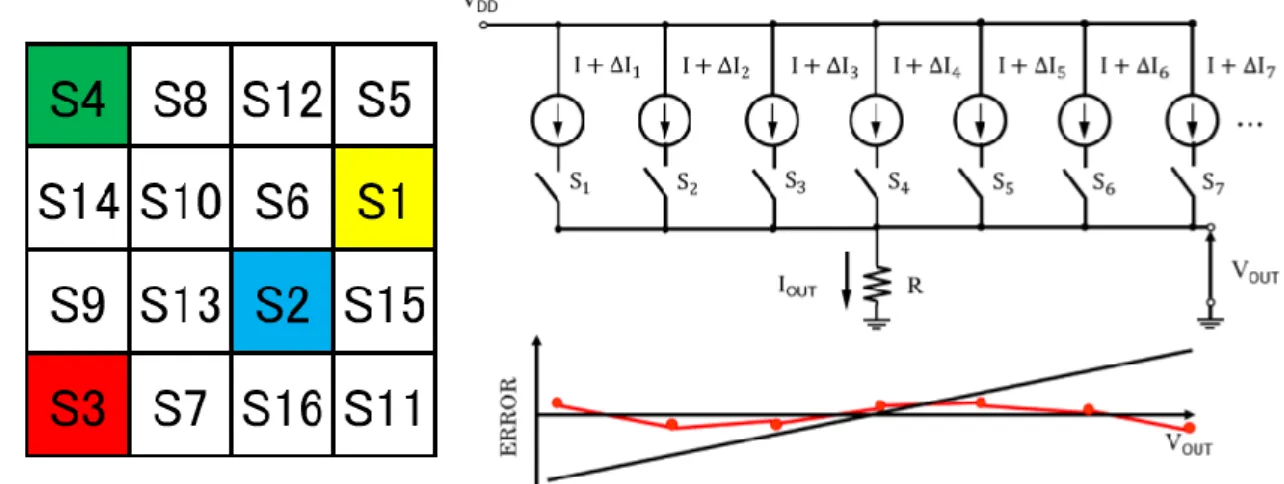
these unit cell outputs. Fig. 2 shows a unary DAC with unit current sources, which is
turned on according to the corresponding decoded digital data. Then, the digital input
is converted into an analog output.
The unary type has less influence on the output signal than the binary type even if
there are mismatches among elements. The glitch is small and monotonicity
characteristics can be guaranteed in principle. However, its disadvantages are large
hardware and power due to a large number of unit cells, as well as conversion speed
restriction to the decoder circuit. When attempting to realize a high linearity DAC, the
relative mismatches among the unit cells (unit currents I in Fig. 2) become a problem.
Fig. 1.Segmented DAC
Fig. 2. Unary DAC circuit and layout of unit cell array.
Many DACs are combinations of unary type and binary type. Unary type with low
sensitivity devices is used for the higher bits, while the binary type with a small
number of elements is for lower bits. Then a high performance DAC with appropriate
circuit scale and power can be realized.
Then we consider only the unary type because the unary type handles higher bits,
2 Circuit Element Characteristics
2.1 Variations in Circuit Element Characteristics
There are systematic variations among MOSFET, resistor and capacitor
characteristics on an integrated circuit, due to their placements, and random variations
which do not depend on their placements. Ideally, the input and output characteristics
of the DAC should be linear. However, in reality due to these variation effects, it
could be nonlinear. The causes of these variations are as follows [2, 9-13].
1) Systematic variations
·Voltage drop on wiring
·Temperature distribution
·CMOS manufacturing process
·Doping distribution
·Changes in threshold voltage
- Accuracy in wafer plane
- Mechanical stress
2) Random variation
· Device mismatch.
The systematic variations can be modeled as linear and quadratic gradients as well
their combination, regarding to the circuit element placements.
· CMOS manufacturing process
2) Quadratic gradient variation
·Temperature distribution
· Accuracy in wafer plane
· Mechanical stress.
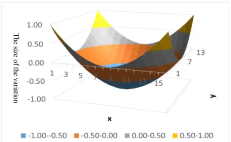
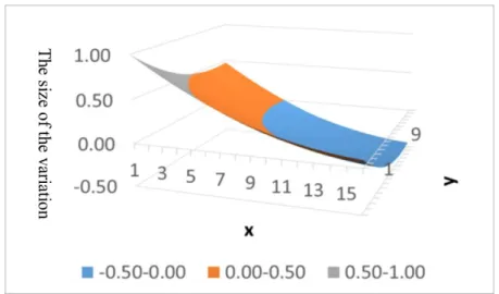
The above variations largely affect the DAC linearity. The variations among the
unit current sources are shown in Figs. 3, 4 and 5. is assumed to be the
coordinates of the position on the chip, and the linear and quadratic variations are
shown by the following expressions.
1) Linear error (Fig. 3)
2) Quadratic error (Fig. 4)
the layout technique for the unit cells. In the case of the segmented DAC, the
variation effects may be reduced by the conventional method (random walk). Then it
also improves the linearity.
Fig. 3. Linear gradient error
Fig. 5. Linear and quadratic joint gradient errors
2.2 Unary DAC Nonlinearity
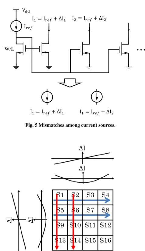
In practical CMOS technologies, the current source mismatches are influenced by
their threshold voltage mismatch and/or by the slope mismatch (Fig.5) [3]. Ideal
drain current Id in saturation region is given by:
Also drain current mismatch is given by;
Current mismatches are dependent on their device sizes. Note that here, we are
considering to reduce the DAC nonlinearity effects of the current mismatches due to
small device size .
These mismatches among current sources may cause the unary DAC nonlinearity
2 1 1 ,2
gs th dV
V
I
WL
t
Av
V
V
I
I
th ox th gs d d 1 1 12
WLdue to their systematic mismatches if they are laid out in a regular manner (Figs.6,
7).
Fig. 5 Mismatches among current sources.
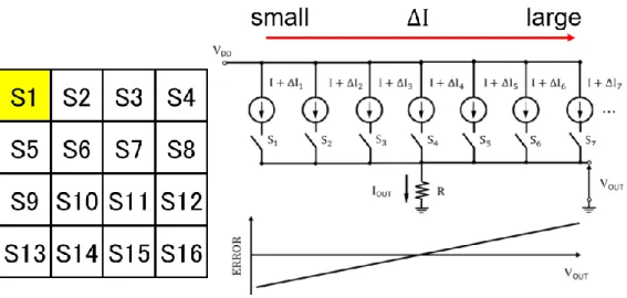
Fig. 6 Regular layout of unit cells for a unary DAC and their linear/quadratic gradient
Fig. 7 Regular layout of unit cells for a unary DAC and its nonlinearity due to their linear gradient errors
3. Magic Square Layout Technique
A magic square has a property that the sums of each row/ column/diagonal element
are all equal. Hence we consider that this property balances the unit cell array of the
unary type DAC, and we have investigated the layout of the unit cells which can
reduce the systematic variation effects to improve the DAC linearity (Fig. 8).
Fig. 8 Layout technique of unit cells for a unary DAC and its linearity improvement by cancelling their linear gradient errors
3.1. Features of Magic Square
The magic square with the n x n matrix, which is arranged in a grid pattern, is a
series of natural numbers starting from 1 to n x n while the numbers on each row,
column or diagonal elements have equal sum [4-6]. Including n elements on each row,
expressed as follows:
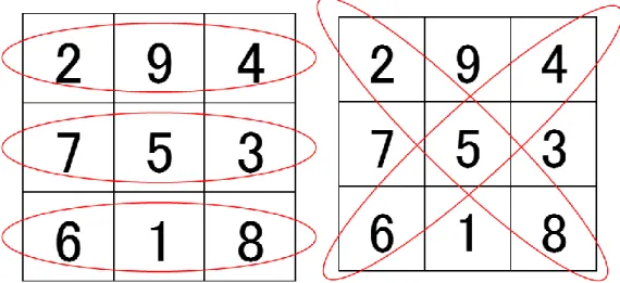
In the magic square shown in Fig. 9, it can be confirmed that the sum of the
elements of each row, column and diagonal components are all equal.
Fig. 9. Equivalent constant sum characteristics.
Utilizing this property, the systematic variations are expected to be reduced by the
magic square layout of the unit cells for a segmented DAC. Even if a concentric
magic square is removed from the outside of the magic square by one side, the
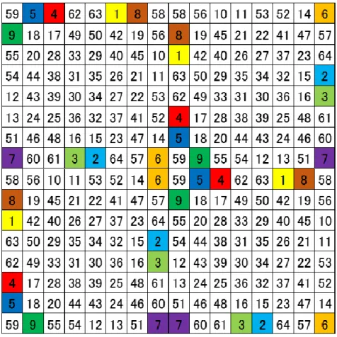
remaining part always does not lose its integrity. The 8-th concentric magic square
used in the analysis is shown in Fig. 10. It is realized by combining four squares with
an 8-bit segmented DAC
3.2. Algorithm Using Concentric Magic Square
symmetry is shown in Fig. 10, and the DAC linearity improvement with the layout
based on the magic square was confirmed by simulation.
Fig. 10. Four 6-bit concentric magic squares
3.3. Analysis Results and Consideration
3.3.1. Linear Gradient Error
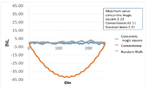
We have examined the linear gradient error case for the unary DAC and its INL
(integral nonlinearity) was examined by simulation for several layout algorithms. We
see that in the linear variation, the concentric magic square was effective to reduce the
Fig. 11. Simulated INL in the linear gradient error case.
3.3.2. Quadratic Gradient Error
In the quadratic gradient error case, the magic square algorithm is effective,
compared to the conventional regular layout algorithm (Fig. 16), and also another
layout algorithm (random walk algorithm [11, 12]) is also effective. (Fig. 12).
3.3.3 Linear and Quadratic Joint Gradient Errors
When the linear gradient variation is larger, the concentric magic square algorithm
will be effective (Fig. 13), and when the quadratic is larger, the random walk is
effective (Fig. 14).
Fig. 13. Simulated INL when the linear gradient error is bigger than the quadratic gradient error.
Fig. 14. Simulated INL when the quadratic gradient error is bigger than the linear gradient error.
4. Latin Square
4.1 Characteristics of Latin Square
Latin squares have n rows and n columns of n different symbols, and are arranged
in such a way that each symbol appears only once in each row and each column (Fig.
15 (a)) [6-8]. Now considering a “complete Latin square”; for even n,put the numbers
1 through n in the first row in the following order:1, 2, n, 3, n-1,…., n/2+2, n/2+1.
(For example, for n=4, we would have 1, 2, 4, 3, …). In each remaining empty cell,
we place the number in the cell directly above it plus 1 (Fig. 15 (b)).
The Latin square was studied by mathematician Leonhard Euler (1707-1783).
Fig.15. (a) 4x4 Latin square (b) 4x4 complete Latin square
4.2Latin Square Layout Algorithm
The linearity of the unary DAC in the variations of the linear and quadratic
regular layout, the common centroid layout (Fig. 17) and the complete Latin square
layout (Fig. 18) are compared.
Fig.16. Regular layout of 2D array of current cells
Fig .17. Common centroid layout of current source Common centroid layout of 2D array of current cells
Fig.18. Standard Latin square layout of 2D array of current cells
The results of numerical simulation INL in case of linear gradient are shown in
Figure 19 and the results INL in case of quadratic gradient error are shown in Figure
20. It can be seen that the Latin square and the common centroid method are almost
equal linearity.
Fig .20. Simulated INL in case of quadratic gradient error
The linearity of the unary DAC in the variations of the linear and quadratic gradients,
is degraded in the regular layout (Fig. 21) in case of 8-bit (16 × 16). This regular
layout, the common centroid layout (Fig. 22) [10, 11, 12] and the complete Latin
square layout (Fig. 23) are compared.
We have simulated static and dynamic performances of an 8-bit unary DAC, and
comparison among the regular layout, the common centroid layout and the complete
Latin square layout was performed. The static performance was simulated as INL and
DNL (Figs. 24-25). The simulated dynamic performance was obtained as Spurious
Free Dynamic Range (SFDR) [1, 2] (Figs. 26-28); there mismatch of current sources
was generated as a random number between -1 from +1. We see that the DAC with
the Latin square algorithm improved SFDR.
The numerical simulation results in the linear gradient variation case are shown in
almost equal linearity.
Fig. 21. Regular layout of 2D array of current cells
Fig. 22. Common centroid layout of 2D array of current cells
Fig. 23. Complete Latin square layout of 2D array of current cells
1 3 6 7 15 9 12 13 4 5 8 2 10 11 14 16 3 2 4 5 8 16 10 11 6 7 1 9 12 13 15 14 6 4 2 3 5 7 16 9 8 1 10 12 14 15 13 11 7 5 3 1 4 6 8 15 2 9 11 13 16 14 12 10 15 8 5 4 1 3 6 7 10 11 14 16 13 12 9 2 9 16 7 6 3 2 4 5 12 13 15 14 11 10 1 8 12 10 16 8 6 4 2 3 14 15 13 11 9 1 7 5 13 11 9 15 7 5 3 1 16 14 12 10 2 8 6 4 4 6 8 2 10 12 14 16 1 3 5 7 15 9 11 13 5 7 1 9 11 13 15 14 3 2 4 6 8 16 10 12 8 1 10 11 14 15 13 12 5 4 2 3 6 7 16 9 2 9 12 13 16 14 11 10 7 6 3 1 4 5 8 15 10 12 14 16 13 11 9 2 15 8 6 4 1 3 5 7 11 13 15 14 12 10 1 8 9 16 7 5 3 2 4 6 14 15 13 12 9 1 7 6 11 10 16 8 5 4 2 3 16 14 11 10 2 8 5 4 13 12 9 15 7 6 3 1
Fig. 24. INL in the linear gradient error case.
Fig. 25. DNL in the linear gradient error case.
Fig. 27. SFDR in the common centroid layout case.
5. Conclusion
In this research, we devise an improvement that magic square and Latin square
layout algorithms are used for the layout algorithms among unit cells to improve the
linearity of a segmented DAC by suppressing their systematic mismatch effects.
Pseudo random numbers are reproduced by the arrangement of the magic square and
Latin square. In addition, it is indicated that the linearity can be improved more than
the conventional technique.
We expect that since there are a lot of magic squares and Latin squares with useful
properties and their mathematical research results, the layout algorithms using them
II. Improve the performance of Two-stage Savonius
wind turbines
1. Introduction
Energy is the backbone of the world economy and a means for progress in the
industrialization of most countries.Energy is directly related to the national economy.
Wind energy is one of the cleanest of energy sources. The energy from wind is
extracted via wind turbines. Offshore wind power generation is attracting attention as
a new energy source in Japan. In the current situation of offshore wind power
generation, the propeller type of the horizontal axis which has been proven in the
wind power generation of the land is mainly used. The propeller type can convert
wind energy to kinetic energy with high efficiency. And it is proven technology.
However, long propeller and heavy nacelle cause unstable structure.
In this research, vertical axis wind turbines are investigated. They are suitable for
offshore in terms of structural stability. The goal of this research is to introduce
vertical axis wind turbines to offshore. Vertical axis wind turbines are not popular
compared to propeller type. In particular, starting characteristics are not investigated.
A vertical axis wind turbine was modified to improve the starting and dynamic
2. Background and Purpose of Research
In addition to the horizontal axis type wind turbine, there are various forms of wind
power generation as shown in Fig.1. Several wind turbines are shown in Fig. 2. They
are roughly divided into a horizontal axis wind turbine and a vertical axis wind
turbine in the direction of the rotation axis. Furthermore, they can be divided into a
lift type that rotates using lift and a drag type that rotates using drag.
Fig.1. Classification of wind turbine type
(B)Vertical axis wind turbine. Fig.2. Wind turbine type
2.1 Horizontal Axis Wind Turbine
In the horizontal axis type, wind turbine has an upwind system in which the
rotating surface of the rotor is located on the upwind side of the tower and a
downwind system on the leeward side.
In the upwind system, since the rotor is located on the windward side of the tower,
it is not affected by the wind turbulence caused by the tower, and the upwind system
is the mainstream of the current wind turbine. On the other hand, the downwind
method has the feature that the yaw drive device for automatically adjusting the
propeller direction to the wind direction is unnecessary. While in the U.S. wind
turbine development stage, a downwind wind turbine is introduced. To the small wind
turbine, although there are not many examples of applications, downwind wind
turbines with large aircraft have also been developed in recent years [1]. The
horizontal axis wind turbines are characterized by the following four.
・Horizontal axis type wind turbines are suitable for power generation.
・In the case of the upwind system, it is necessary to direct the rotating surface of the wind turbine to the wind (yaw control).
・It is necessary to install heavy objects (generator, transmission mechanism, control mechanism, etc.) in the nacelle.
2.2 Vertical Axis Wind Turbine
Next, four features are listed as characteristics of the vertical axis wind turbine.
・Wind in any direction is available and there is no dependence on wind direction. ・Heavy materials can be installed on the ground.
・Manufacture of blades is easier than propeller type.
・Compared with horizontal axis wind turbine, its efficiency is low and setting area is large.
2.3 Lift Type and Drag Type Wind Turbine
As a classification according to the working principle, wind turbines are divided
into a lift type and a drag type. Lift type is efficient and suitable for power generation,
since it can rotate at high speed at higher than the wind speed. However, a large
torque is required at the time of self-starting, and the rotational speed control is
difficult. On the other hand, drag type cannot rotate at high speed. But a large torque
2.4 Savonius Wind Turbine
Savonius wind turbine which is one of a vertical axis drag type wind turbine is
focused in this study. This is because, when considering installation on the ocean,
vertical axis type stability is an advantage. Savonius wind turbine was invented by
Finnish engineer Savonius in 1924 [2]. It consists of two half cylinders as shown in
Fig. 3.
Fig.3. Diagram of Savonius wind turbine
Savonius wind turbine has a shape in which a hollow cylinder is cut in half and
ends are connected through a rotating shaft. A sectional view of the Savonius wind
turbine is shown in Fig4. It is an effective wind turbine that rotates with the force
pushing the blade of the wind turbine. As shown in Fig. 4, by shifting the blades
inward and providing overlapping portions, a part of the wind received by the blade
on the upper side of the drawing flows into the other blade (the lower side in the
figure) through the gap. This improves efficiency. According to the overlap, the
wind turbine radius [3]. This study is to investigate the basic characteristics, as much
as possible using a wind turbine whose shape is as simple as possible. In other words,
the overlap ratio is 0.
Fig.4. A Sectional view of Savonius wind turbine
Savonius wind turbine receives the wind in the concavity of the blade and the wind
rotates with the force pushing the blade. When the blade is in the position shown on
the left of Fig. 5, the upper blade has wind resistance to wind, while the wind escapes
the lower blade. Therefore, a difference in drag occurs between the two blades, and
the wind turbine rotates clockwise.
However, when the wind direction and the wind turbine are in the positional
relationship as shown on the right side of Fig. 5, the wind is difficult to enter the blade,
so the force in the direction to rotate the wind turbine becomes small. As a result, the
force in the direction of pushing back the blade relative to the blade on the lower side
of the figure relatively increases, so that a negative torque, that is, a force rotating in
the opposite direction, is generated.
As mentioned in Section 2.2 and 2.3, it is a major feature of the Savonius wind
and the blade becomes difficult to start and rotate [4]. Therefore, the purpose of this
research is to improve Savonius wind turbine so that it is easy to start and rotate.
Fig.5. Mechanism of rotation of Savonius wind turbine
2.5 Improvement of Savonius Wind turbine
In order to improve the difficulty of starting due to the wind coming from a specific
direction and the large variation of torque during rotation, several improvements have
been carried out. Fig.6 shows some examples; Savonius wind turbine with multi-layer
superposition, blade and screw, and guide vanes installation.
(a) Multistage type (3 stage) (b) Multistage type (2 stage)
Hybrid with Darius Wind turbine
(c) Torsion type Hybrid with solar power
(d) Torsion type (e) Installation of guide vanes
Fig.6.Improvement of Savonius wind turbine
In this research, we aim to the improvement of the startability and suppress torque
fluctuation during rotation, and improve wind turbines like multi-stage (two-stage)
wind turbines as shown in Fig. 6 (b). According to the symmetry of its shape, the
upper stage of the 2-stage wind turbine in Fig.6 (b) is shifted 90 degrees from the
lower stage and stacked. In the same way, each stage of 3-stage wind turbine in Fig.6
(a) is shifted 60 degrees with each other. However, it has not been verified if it is the
best shape. Numerical experiments are carried out on several wind turbines with
different deviation angles in the second segment, and the analysis of their
characteristics (static torque and dynamic torque) and the exploration of the optimal
shape are carried out.
Fig.7. Multistage (two-stage) wind turbines
(in the order from left, upper stage is shifted 0 degree, 30 degrees, 60 degrees, 90 degrees, from lower stage)
3. Numerical Solution
Numerical simulation is effective when searching for the optimum shape of the
wind turbine blade. One of the reasons is that it is easy to calculate by changing the
shape of the wind turbine and the conditions of the flow field. In addition, as a
preliminary stage to the experiment, numerical simulation is effective. By observing
the visualized flow field, the formation of characteristic vortices when the wind speed
changes, and the observation of pressure field, we can confirm the characteristic of
the wind turbine. In this section, we describe a solution method of numerical
simulation performed on the flow around the wind turbine.
3.1 Calculation Area and Boundary Condition
As shown in Fig. 8, the computation area was a cylindrical shape with the wind
turbine enlarged to the outside, and a non-uniformly spaced grating which became
rougher as going away from the wind turbine was used. The number of grids was set
to circumferential direction 72 × radial direction 60 × height direction 80.
Boundary conditions imposed a uniform flow at the far boundary, free flowing
condition at the top and bottom of the calculation area. And no-slip condition was
employed on the wind turbine blade. As the shape of the wind turbine, as shown in
Fig. 9, there is no overlap ratio, and the tip of the blade is in contact with the rotation
axis. A Savonius wind turbine having no overlap ratio is sometimes called an
S-shaped rotor from its shape. The blade shape is an ellipse with a length of 1.0 and a
radius is 1.0, the bucket depth is 0.4. As shown in Fig. 8, the aspect ratio of the wind
turbine as a whole was fixed at 1.0 wind turbine diameter and 2.0 wind turbine height.
Fig.8. Calculation area Fig.9.Blade section
3.2 Coordinate System
In this study, we assume that the wind turbine is rotating around the axis at a
constant angular velocity, and uses a rotating coordinate system fixed to the wind
turbine blade. Assuming that the rotation angle measured from the stationary state is
t
between the rotating coordinate system (X,Y,Z) and the stationary coordinate system(x,y,z), there is the following relationship.
Coordinate transformation
sin cos Y X x Z z Speed transformation sin cos y x X cos sin Y X y Y xsin ycos y V Uu cos sin U ucos
vsin
Yx
V
U
Operator Stationary coordinate Rotational coordinate Dt D z w y v x u t Z W Y V X U t 2 2 2 2 2 2 2 z y x 2 2 2 2 2 2 Z Y X grad x sin cos Y X y cos sin Y X div v z w y v x u Z W Y V X U
Fig.10. Stationary coordinate system and rotating coordinate system
3.3 Basic Equation
The basic equation is shown in the rotating coordinate system as follows.
Equation of continuity:
0
Z
W
Y
V
X
U
Equation of motion (incompressible Navier-Stokes equation)
t:time, :pressure, : Reynolds number based on the radius of the rotor and
the uniform flow (in this study, Re is set as 105). After converting fundamental
equations to general coordinates, the calculation is performed by using the fractional
step method described later.
3.4 General Coordinate Transformation
In order to accurately impose the boundary condition along the wind turbine blade,
the grid is complicated because it uses a grid along the blade as shown in Fig. 9.
Therefore, the transformation function is used to transform the three-dimensional
coordinates into an orthogonal grid (computational plane) [5 (Chapter 5.4)]. Fig. 10 is
a conceptual diagram. 2 2 2 2 2 2 2 Re 1 2 Z U Y U X U X p V X Z U W Y U V X U U t U 2 2 2 2 2 2 2 Re 1 2 Z V Y V X V Y p U Y Z V W Y V V X V U t V 2 2 2 2 2 2 Re 1 Z W Y W X W Z p Z W W Y W V X W U t W p Re
Fig.11. Coordinate transformation
3.5 Fractional Step Method
In this study, we use a fractional step method [6] to solve the Navier-Stokes
equations. This is a method of separating the viscous term from the pressure term by
using the intermediate velocity (temporary velocity).
𝛿𝑡:Time step width (constant), = (0,0, ), =( , ,0), =( , , ), If n
v represents the n-th step ofv , the incompressible Navier-Stokes equation is approximated by the intermediate velocity v* like (3.5.1).
n n n n n t v v v r v v v ω ω ω ( ) 2 Re 1 ) ( * 2
(3.5.1)Formula (3.5.1) is transformed into formula (3.5.2). With given v0 as the initial value, the intermediate velocity v* is derived by calculating the right side of (3.5.2).
(3.5.2)
Although the original Navier-Stokes equation is partly replaced by the equation
(3.5.1), the equation (3.5.3) still can be derived from taking the divergence of both
ω r X Y v U V W } 2 ) ( Re 1 ) ( { * vn t vn vn 2vn r vn v ω ω ω
sides and substituting the continuous equation.
(3.5.3)
Equation (3.5.4) is derived from the original Navier-Stokes equation by substituting
the intermediate speed equation (3.5.1).
(3.5.4)
By repeating the equations (3.5.2) - (3.5.4), time development is carried out and the
solution can be obtained as shown in Fig12.
Fig.12. Fractional step method
3.6 Difference
The time derivative is approximated by using the forward differences shown in
(3.6.1). Spatial derivative other than nonlinear term is approximated by using the
central differences shown in (3.6.2).
*) ( 1 1 2 v t Pn
1 1*
n nP
t
v
v
t
u
u
t
u
n n n t
1 (3.6.1) x u u x u i i xi x 2 1 1 (3.6.2)When approximating a nonlinear term, using central differences when computing a
flow with a large Reynolds number with a coarse grid becomes numerically unstable.
However, even when the grid is not sufficiently fine, it is possible to calculate stably
using the third-order upwind differences [7].The upwind differences of the third order
accuracy is an approximation expression using four points weighted upstream as in
equation (3.6.3). x u u u u f x u f x xi i i i i (2 1 3 6 1 2) 6 ( f 0) x u u u u f( i2 6 i1 3 i i1) 6 ( f 0) (3.6.3)
Equation (3.6.3) can be summarized into one expression as shown in equation
(3.6.4) if absolute values are used.
4 2 1 1 2 3 2 1 1 2 4 6 4 12 12 ) ( 8 x u u u u u x f x u u u u f x u f i i i i i i i i i xi x (3.6.4)
Note that u represents the value of ui at pointx . In this section, it is explained i
Fig.13. Points around xi
3.7 Definition of the shape of the wind turbine
The bucket which moves on the side of proceeding direction is called as
"advancing bucket" and the bucket which moves on the side of opposite direction is
called as "returning bucket". As shown in Fig. 14, when uniform flow is blowing from
the left direction, the bucket on the upper side of the figure becomes the "advancing
bucket" and the lower side bucket becomes the "returning bucket". If the wind turbine
rotates 180 degrees, the bucket currently in the position of the advanced side becomes
the return side bucket this time.
The displacement angle of the second stage wind turbine with respect to the first
stage wind turbine is called Phase (phase angle), and it is expressed in ∅.As shown in FIG. 15, the second stage wind turbine is shifted with reference to the first stage.
When∅ = 0, it means a conventional, undeformed Savonius wind turbine. According to the symmetry of wind turbine shape, ∅ is defined only between 0 and 90 degrees.
Calculate the torque (static torque) generated when the wind blow around the fixed
wind turbine blade to investigate the self-starting ability of the wind turbine. "Attack
elapsed since the start of calculation is considered as the static torque. Since the wind
turbine shape is a 180 degree cycle, attack angle is defined only between 0 and 179
degrees.
Fig.14. Position relationship between blade and wind
Fig.15. Define of phase(2-stages degree)
3.8 Parameters for Wind Turbine Output
When evaluating the performance of wind turbine, the following characteristic
coefficients with generality are used.
T:Torque (the force with which the wind turbine rotates).
It is the force applied to the blade multiplied by the distance from the center
of the rotating shaft to the point of application of force. Because it is a
product of force and distance, it becomes the same unit as work.The
calculation method is described later. (See section 3.9)
Ct :Torque coefficient(Ct T/qRA)
Ct is non-dimensionalized T by the size of the wind turbine.
q:dynamic pressure(/2),:air density,R:radius of the turbine,
A :the sweep area of the blade (assuming H is the rotor height, A RH).
:Tip speed ratio(R/u)
The tip-speed ratio for wind turbines is the ratio between the tangential speed
of the tip of a blade and the actual speed of the wind. The tip-speed ratio is
related to efficiency, with the optimum varying with blade design. Higher tip
speeds result in higher noise levels and require stronger blades due to large
centrifugal forces.
Percentage of energy that wind turbines can extract from the wind. It shows
how much work was done per unit time.It shows the performance of the
wind turbine.
3.9 Calculation of Torque
Torque T generated by wind turbine is calculated according to the pressure
difference between the front and the back of wind turbine blade in each micro area on
the blade.
By calculating the fluid by the method described in section 3.1 - 3.6, the pressure at
each grid point is obtained. The torque involved in the micro area of Fig. 17 (a) can be
calculated according to the following formula.
r p p x T w in out ( )
As shown in Figure 17(b), the rotational component of is the torque associated T
with the micro-region. Similarly, calculations are performed for all areas on the blade,
(a) Torque applied to the
blade
(b) Component of rotation direction of torque Fig.17. Calculation of torque
4. Results and Considerations
As shown in section 2.4, the Savonius wind turbine generates negative torque when
it receives wind from a certain direction, and it is hard to start and rotate. In order to
eliminate the portion where negative torque is generated and make it easier to start
and rotate, we tried overlapping Savonius wind turbines in two stages and examined
how the torque generated by shifting the wind turbine angle changes.
4.1 Self-starting Characteristics of Wind Turbine
Self-starting characteristics is shown in Fig. 18. The horizontal axis of the graph of
Fig. 18 is the angle of attack which is the angle of the wind corresponding to the fixed
wind turbine defined in Section 3.7, and the vertical axis is the torque coefficient Ct of static torque which is the force to start to rotate the wind turbine as defined in
Section 3.8. If Ct is large, the self-starting characteristics are good. In other words, the wind turbine can start to rotates easily. If Ct is negative, the wind turbine cannot start to rotate. The characteristics are compared by the phase of 2 stage. The phases of
2 stage are changed from 0 to 90 degrees, and the characteristics are compared.
First, the results of Fig.18.(a) is described. It is the original Savonius wind turbine,
the phase ∅ angle is 0 degree. The value of the torque coefficient Ct is large when α is around 50 to 60 degrees while it becomes negative at 140 to 170 degrees, so that the
wind turbine cannot be started.We can see that wind is more likely to enter the
advancing bucket when α is around 50 to 60 degrees. While α is around 160 degrees, the wind is blowing in such a direction, that is opposite to the rotation
direction of the wind turbine, to push the returning bucket. This is also consistent with
the mechanism of rotation of the Savonius wind turbine explained in Section 2.4.
Next, in order to investigate how much the stationary torque improves by rotating
the second stage with respect to the first stage and shifting the phase, the stationary
torque is calculated for the ten kinds of wind turbines with different phase angles by
10 degrees (Fig.18(b)-(j)). As an example, the results of Fig.18.(j) is described as an
example. In the region of attack angle of 140 to 170 degrees, the first stage of wind
turbine indicated by blue line in Fig. 19 cannot produce positive torque. While the
second stage of wind turbine indicated by red line can produce positive torque.
Similarly, at attack angle of 40 to 70 degrees at which the second stage wind turbine
cannot generate a positive torque, the first stage wind turbine generates a positive
torque. As a result of summing the torque coefficients of the two stages, as shown by
the green line, it can be seen that the wind turbine as a whole produces positive torque
regardless of what angle the wind blows. Thus, it can be considered that the portion
where the static torque becomes negative can be canceled by overlapping the first
stage and the second stage, thereby eliminating the area that cannot be started. As
shown in Fig. 18, negative torque does not occur when modified by the phase ∅ angle is 60 degrees or more.
(a) ∅=0 (b) ∅=10
(c) ∅=20 (d) ∅=30
(e) ∅=40 (f) ∅=50
(i) ∅=80 (j) ∅=90 Fig.18. Comparison of self-starting characteristics of wind turbines
4.3 Dynamic Characteristics of Wind turbine
Next, we investigate the characteristics (dynamic characteristics) during wind
turbine rotation.Figure 19 (a) shows the time variation of the torque coefficient of the
original wind turbine (phase angle ∅ = 0) The turbine rotated at a constant tip speed ratio λ=0.5, that is, when the tip of blade moves at the speed of half of the wind speed. The horizontal axis of the graph is the rotation angle measured from the stationary
state, and the vertical axis θ is the torque coefficient.θ is the change in torque factor between 720 degrees and 1,080 degrees.It can be seen from the symmetry of the shape
of the wind turbine that it has a period of 180 degrees. In the pre-deformation wind
turbine, the fluctuation periods of the torque of the wind turbines of the first and
second stages are the same, and the fluctuation of the torque of the wind turbine as a
whole is also large.
On the other hand, in the modified wind turbine (phase angle ∅ = 90 ) shown in Fig. 19 (b), the fluctuation periods of the torques generated by the wind turbines of
total torque coefficient is smoothed.It is considered that the smoothness of the
variation of the torque coefficient improves the durability of the wind turbine.
(a) Wind turbine before deformation(Phase angle 0)
(b) Wind turbine after deformation(Phase angle 90)
Fig.19. Time variation of the torque coefficient of the wind turbine
4.4 Flow Field around Wind Turbine
Fig. 22 shows contour lines of vorticity at the center section of the wind turbine.
They are flow fields with the attack angle at which the largest torque is generated. In
is seen that the wind turbine is swept down the leeward side (the right side in the
figure) on the wind.
(a) 2-stages degree=0 Attack angle=40 (b) 2-stages degree=10 Attack angle=40
(e) 2-stages degree=40 Attack angle=60 (f) 2-stages degree=50 Attack angle=80
(g) 2-stages degree=60 Attack angle=80 (h) 2-stages degree=70 Attack angle=80
(i) 2-stages degree=80 Attack angle=100 (j) 2-stages degree=90 Attack angle=120 Fig.22. Flow around the wind turbine
5. Conclusion and Discussion
5.1 Conclusion and Discussion
In this study, improvements were made to Savonius wind turbine which is one of
the vertical axis drag type wind turbines in order to improve the start ability and
reduce the variation of the torque coefficient during rotation. As a result of numerical
simulation, we found the following for the two-stage Savonius wind turbine with
different phase angles.
In the wind turbine before the deformation, the stationary torque is negative against the specific wind direction, so it is difficult to start to rotate
Applying a phase angle to the second stage wind turbine smoothest the torque, and when the phase angle is 60 degrees or more, the stationary torque can be
made positive for all wind directions, leading to improved start ability
Dynamic characteristics degrade as the phase angle of the wind turbine increases. However, due to the smoothed torque fluctuation during the rotation, it is
effective in improving the durability of the wind turbine.
Considering both starting characteristics and dynamic characteristics, the best phase angle will be 60 degrees.
5.2 Future Issues
It is concerned that a nonpoint symmetrical shape with a phase angle of 60 degrees
Also, the flow field becomes complicated as the wind turbine shape becomes
complicated. In order to investigate the characteristics of the wind turbine,
three-dimensional analysis of the flow field is indispensable. It is necessary to study
References
I. Improve Linearity of DA Converter
[1] F. Maloberti, Data Converters, Spring (2007),
[2] R. V. D. Plassche, Integrated Analog-to-Digital and Digital-to-Analog Converters,
Springer (2012).
[3] M. J. M. Pelgrom, AAD C. J. Duinmaijer, A. O. G. Welbers, “Matching Properties
of MOS Transistors”, IEEE Journal of Solid-State Circuits, vol. 24, no.5 ,
pp.1433-1440 (Oct. 1989).
[4] K. Omori, The World of Magic Square, Nippon Hyoron Sha, Japan (Aug 2013).
[5] H. Sato, Geometry Magic-Modern Mathematics From the Magic Square, Nippon
Hyoron Sha, Japan (2002).
[6] T. Omura, Story of Mathematical Puzzle, Union of Japanese Scientists and
Engineers (1998).
[7] M. Yoshizawa, How to Take a Problem, How to Use Practical Application,
Maruzen (2012).
[8] W. L. Stevens, “The Completely Orthogonalized Latin Square”, vol. 9, no. 1,
82-93 (Jan 1939).
[9] T. Miki, Y. Nakamura, M. Nakaya, S. Asai, Y. Akasaka, Y. Horiba., "An 80-MHz
8-bit CMOS D/A Converter”, IEEE Journal of Solid-State Circuits, vol. 21, no. 6,
pp.983- (Dec. 1986).
Journal of Solid-State Circuits, vol. 34, no. 12, pp. 1708-1718 (Dec. 1999).
[11] Y. Cong, R. L. Geiger, “Switching Sequence Optimization for Gradient Error
Compensation in Thermometer-Decoded DAC Arrays”, IEEE Trans. Circuits and
Systems II, vo. 47, no. 7, pp.585- 595 (July 2000)
[12] K.-C. Kuo, C. –W. Wu, “A Switching Sequence for Gradient Error Compensation
in the DAC Design”, IEEE Trans. Circuits and Systems II, vol. 58, no. 8, pp. 502-506 (Aug 2011).
[13] X. Li, F. Qiao, H. Yang,“Balanced Switching Schemes for Gradient-Error
Compensation in Current-Steering DACs”, IEICE Trans. Electron, vol. E95-C, no.11,
pp. 1790-1798 (Nov. 2012).
[14] M. Higashino, S. N. B. Mohyar, H. Kobayashi, “DAC Linearity Improvement
Algorithm With Unit Cell Sorting Based on Magic Square”, IEEE International Symposium on VLSI Design, Automation and Test, Hsinchu, Taiwan (April, 2016).
II. Improve the performance of Two-stage Savonius wind turbines
[1] 福 島 大 学 「 風 力 発 電 シ ス テ ム 概 論 」
(http://www.sss.fukushima-u.ac.jp/saiene/lecture/8) [2] Savonius, S.J.: Mech. Eng., Vol. 53, No. 5, (1931), p333.
[3] Izumi USHIYAMA and Hiroshi NAGAI: Optimum Design Configurations and
Performance of Savonius Rotors, Wind Eng., Vol. 12, No. 1, (1988), pp. 59-75.y,
Japan
計算(放出渦が運転特性に及ぼす影響)”, 機械学会論文集, 61-581, B(1995-1), pp. 12-17.
[5] 河村哲也「流体解析Ⅰ」朝倉書店 (1996)
[6] Yanenko, N.N.: The method of fractional steps, Springer-Velag, (1971).
[7] Kawamura, T. and Kuwahara, K: Computation of high Reynolds number flow
Research Achievements
[1] Haruo Kobayashi, Yuto Sasaki, Hirotaka Arai, Dan Yao, Yujie Zhao, Xueyan Bai,
Anna Kuwana, “Unified Methodology of Analog/Mixed-Signal IC Design Based on
Number Theory”, IEEE 14th International Conference on Solid-State and Integrated Circuit Technology, Qingdao, China (Nov. 2018) (IEEE Xplore)
[2] Dan Yao, Anna Kuwana and Haruo Kobayashi Gunma University, Japan
"Numerical Simulation for Characteristic Analysis of Vertical Axis Wind Turbine",
5th International Symposium of Gunma University Medical Innovation and 9th
International Conference on Advanced Micro-Device Engineering, Dec. 6, 2018
Kiryu City Performing Art Center
[3] Richen Jiang, Gopal Adhikari, Yifei Sun, Dan Yao, Rino Takahashi,Yuki Ozawa,
Nobukazu Tsukiji, Haruo Kobayashi, Ryoji Shiota, “Gray-code Input DAC Architecture for Clean Signal Generation”, IEEE International Symposium on
Intelligent Signal Processing and Communication Systems (ISPACS), Xiamen, China
(Nov. 6-9, 2017).IEEE Xplore
[4] Dan Yao, Yifei Sun, Masashi Higashino, Shaiful Nizam Mohyar, Tomonori
Yanagida, Takuya Arafune, Nobukazu Tsukiji, Haruo Kobayashi, “DAC LINEARITY IMPROVEMENT WITH LAYOUT TECHNIQUE USING MAGIC AND LATIN
Communication Systems (ISPACS), Xiamen, China (Nov. 6-9, 2017).IEEE Xplore
[5] Yifei Sun, Shu Sasaki, Dan Yao, Nobukazu Tsukiji, Haruo Kobayashi "Study on
Digital Multiplier Architecture Using Square Law and Divide-Conquer
Method".International Conference on Mechanical, Electrical and Medical Intelligent
System 2017 (ICMEMIS2017) Nov. 29, 30 & Dec. 1, 2017 (Kiryu, Japan)
[6]佐々 木秀, 孫 逸菲, 姚 丹, 小林 春夫「2 乗則を用いたデジタル乗算器の 研究」第 7 回 電気学会東京支部栃木・群馬支所 合同研究発表会 於 足利工業 大学 2017 年 3 月 2 日(木),3 月 3 日(金) [7] 姚 丹, 孫 逸菲, 東野 将史, 荒船 拓也, 小林 春夫 .「ラテン方陣,魔方陣 レイアウトアルゴリズムを用いた DA 変換器線形性向上」 (レイアウトの重要 性)第 7 回 電気学会東京支部栃木・群馬支所 合同研究発表会於 足利工業大 学 2017 年 3 月 2 日(木),3 月 3 日(金)
Acknowledgments
I would like to express my deepest gratitude to Professor Haruo Kobayashi for his
encouraging guidance and encouragement in promoting this research. I was involved
in research on improving the linearity of the DA converter, and received many
opportunities. In particular, such as presentations at International Association IEEE –
2017Through research, I learned how to look and think about things, and the words
"job fee is work" are inscribed in my mind. Thanks to assistant professor Anna
Kuwana, I receive the professor of research many times and thank you. I thank you
from the bottom of my heart for becoming extremely helpful and became a major
guideline for research.First of all let's get used to the everyday life in Kiryu.Ishikawa
Nobuyuki I thank you from the bottom of my heart for helping the technical staff
from research life to job hunting.
Thank you for my family who watched me warmly until graduation and
completion.
After entering Gunma University, I joined Kobayashi Laboratory and took up a
position in this enterprise. I never thought of such a thing. It must be fate. We will