Trade, Exchange Rates, and Macroeconomic
Dynamics in East Asia: Why the Electronics
Cycle Matters
著者
Kumakura Masanaga
権利
Copyrights 日本貿易振興機構(ジェトロ)アジア
経済研究所 / Institute of Developing
Economies, Japan External Trade Organization
(IDE-JETRO) http://www.ide.go.jp
journal or
publication title
IDE Discussion Paper
volume
34
year
2005-08-01
INSTITUTE OF DEVELOPING ECONOMIES
Discussion Papers are preliminary materials circulated
to stimulate discussions and critical comments
Abstract
Against the background of increasing regional trade and investment, there is growing
interest in monetary and macroeconomic policy coordination in East Asia. Although
there is a sizable literature on macroeconomic linkages among East Asian countries and
the potential merit of policy coordination in the region, the existing studies tend to
examine these issues exclusively in terms of macroeconomic variables and do not
consider how these aggregate variables are influenced by one prominent feature of a
number of East Asian economies: their heavy dependence on the electronics industry.
Although active engagement in the global electronics industry has been a powerful
growth engine for the Asian countries, it has also left their economies vulnerable to
cyclical fluctuations in the world electronics market. As the cycle of the global
electronics industry exerts profound impacts on the medium-term dynamics of the Asian
economies, it is imperative to take an explicit account of its influence when studying the
way in which the regional economies are linked to one another and how this
relationship can be altered by a specific policy initiative. We illustrate the importance of
this point by examining recent studies on: (1) trade competition between China and
DISCUSSION PAPER No. 34
Trade, Exchange Rates, and
Macroeconomic Dynamics in East
Asia: Why the Electronics Cycle
Matters
other Asian countries and the role of the Chinese renminbi therein; and (2) the effect of
fluctuations in the yen/dollar exchange rate on the regional economies.
Keywords: electronics cycle, export competition, renminbi, yen/dollar exchange rate
JEL classification: F14, F15, F33, F440
* Associate Professor, Graduate School of Economics, Osaka City University and Visiting Research Fellow, Development Studies Center, Institute of Developing Economies ([email protected] / [email protected])
The Institute of Developing Economies (IDE) is a semigovernmental,
nonpartisan, nonprofit research institute, founded in 1958. The Institute
merged with the Japan External Trade Organization (JETRO) on July 1, 1998.
The Institute conducts basic and comprehensive studies on economic and
related affairs in all developing countries and regions, including Asia, Middle
East, Africa, Latin America, Oceania, and East Europe.
The views expressed in this publication are those of the author(s). Publication does not imply endorsement by the Institute of Developing Economies of any of the views expressed.
INSTITUTE OF DEVELOPING ECONOMIES (IDE), JETRO 3-2-2, WAKABA,MIHAMA-KU,CHIBA-SHI
CHIBA 261-8545, JAPAN
TRADE, EXCHANGE RATES, AND MACROECONOMIC DYNAMICS IN
EAST ASIA: WHY THE ELECTRONICS CYCLE MATTERS
*Masanaga Kumakura
†August 15, 2005
AbstractAgainst the background of increasing regional trade and investment, there is growing interest in monetary and macroeconomic policy coordination in East Asia. Although there is a sizable literature on macroeconomic linkages among East Asian countries and the potential merit of policy coordination in the region, the existing studies tend to examine these issues exclusively in terms of macroeconomic variables and do not consider how these aggregate variables are influenced by one prominent feature of a number of East Asian economies: their heavy dependence on the electronics industry. Although active engagement in the global electronics industry has been a powerful growth engine for the Asian countries, it has also left their economies vulnerable to cyclical fluctuations in the world electronics market. As the cycle of the global electronics industry exerts profound impacts on the medium‐term dynamics of the Asian economies, it is imperative to take an explicit account of its influence when studying the way in which the regional economies are linked to one another and how this relationship can be altered by a specific policy initiative. We illustrate the importance of this point by examining recent studies on: (1) trade competition between China and other Asian countries and the role of the Chinese renminbi therein; and (2) the effect of fluctuations in the yen/dollar exchange rate on the regional economies. Keywords: Electronics Cycle, Export Competition, Renminbi, Yen/Dollar Exchange Rate JEL Classification: F14, F15, F33, F42 * The author thanks Masato Kuroko of the Institute of Developing Economies, Japan External Trade
Organization, for providing trade indices compiled as part of its ongoing research project and compiling a few new indices at the request of the author. The author is also grateful to a number of staff economists at the institute for their advice about data on countries of their specialization.
† Associate Professor, Graduate School of Economics, Osaka City University and Visiting Research
1. INTRODUCTION Against the backdrop of the 1997 Asian crisis and increasing regional trade and investment flows, there has been growing interest in monetary and macroeconomic policy coordination in East Asia. According to some authors, monetary policy coordination and joint exchange rate management would help East Asian countries not only to manage their own economies but also to adjust their collective relationship with the rest of the world (Williamson 2005). In recent years, for example, the Asian countries have collectively been incurring a massive trade surplus with the United States while intervening heavily in foreign exchange markets to stave off their currencies’ appreciation. According to some observers, the Asian monetary authorities’ extensive exchange market intervention reflects not so much their desire to keep their currencies pegged to the dollar as their fear of losing export competitiveness to other Asian countries, notably China (Persaud and Spratt 2004). Other authors argue that the uncoordinated exchange rate policies of East Asian countries keep their economies vulnerable to fluctuations in the exchange rates among the world’s major currencies. It is widely perceived, in particular, that large medium‐term swings in the yen/dollar exchange rate changes Japan’s export competitiveness vis‐à‐vis other East Asian economies and generate unnecessary export and macroeconomic fluctuations among the latter (Ogawa and Ito 2002). In the eyes of some authors, these issued can be best dealt with by introducing an explicit regional monetary arrangement and coordinating the interests of individual countries (McKinnon 2005).
The foregoing issues ‐‐ trade competitiveness between China and other East Asian economies, the effect of a renminbi (RMB) revaluation on regional trade flows, the relationship between the yen/dollar exchange rate and emerging Asian economies, the role of trade and exchange rates in regional business cycle transmission – have all been studied extensively in recent years. The existing studies, however, tend to approach these issues exclusively from a macroeconomic perspective, often adopting an analytical framework developed to study macroeconomic interaction among major industrial countries. In consequence, these studies tend to play down structural differences between the emerging East Asian economies and mature industrial economies and their implications for the issues
under investigation.
One prominent feature shared by a number of East Asian economies is their heavy dependence on the electronics industry. Whilst the Asian countries’ active participation in global electronics production networks has helped their rapid industrialization and economic growth, it has also left their economies vulnerable to cyclical fluctuations in the world electronics market. Although the burst of the dotcom bubble in the United States in 2000 and the subsequent global electronics recession have highlighted their structural weakness, the sensitivity of the Asian economies to the world electronics cycle is in fact of much longer standing. Thus any empirical research on the medium‐term dynamics of the East Asian economies and their regional repercussions must recognize this point explicitly. We will illustrate the importance of this point by examining a sample of recent studies on: (1) trade competitiveness between China and other East Asian countries and its implication for China’s exchange rate policy; and (2) the relationship between yen/dollar exchange rate fluctuations and the business cycles of emerging Asian countries. As we will see, many of the apparently strong results in these studies are turned upside down once an explicit account has been taken of the electronics cycle.
The rest of this paper is organized as follows. In the next section, we first provide a broad review of the world electronics industry and its relationship with the East Asian economies. Section 3 looks at recent debate on the competitive relationship between the exports of China and other East Asian countries and factors underlying their medium‐term export performance. In Section 4, we examine recent literature on the relationship between the yen/dollar exchange rate and the business cycles of the Asian economies. Section 5 summarizes the findings of the paper and comments on what needs to be explored further to improve our understanding of the macroeconomic interaction among the Asian countries and its relationship with the world electronics market. In Appendix A, we follow up Section 3 by looking more closely at China’s trade statistics and the implication of the recent change in the country’s exchange rate policy. Appendix B complements Section 4 by providing an additional analysis of the historical relations among the electronics cycle, the export performance of the Asian countries and the external value of their currencies. Appendix C details the data and variables used in our econometric investigation.
2. THE GLOBAL ELECTRONICS CYCLE AND EAST ASIAN ECONOMIES The electronics industry is loosely defined as the industry that produces semiconductor and other electronic devices, as well as industrial, consumer and other end‐user equipment that depends heavily on such devices. During the past three decades, the electronics industry is one of the fastest growing segments of the world economy. Table 1 shows the global output of major electronic products in 1987 and 2002. Not surprisingly, “Electronics Data Processing” (mostly PCs and peripherals) and “Radio Communications and Radar” (increasingly dominated by mobile telephones and related products) represent the two largest end‐user markets. “Components” also constitutes a sizable sub‐category, reflecting the fact that producers of parts and components are a major industry player in their own right and trade with myriads of down‐ as well as up‐stream producers. Researchers and industry analysts frequently refer to the “global electronics industry”, stressing the fact that producers based in any specific country are typically connected through various production sharing arrangements with their foreign subsidiaries and other firms around the world (Ernst 2004).
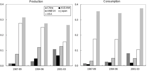
As is widely documented, East Asian countries’ active participation in the global electronics industry has been an important catalyst for their industrialization and integration into the world economy. Figure 1 illustrates how the shares of the United States and ten East Asian countries in the global production and consumption of electronics have evolved over the past two decades. In this figure and throughout the rest of this paper, “ANIES4” refer to Hong Kong, Korea, Singapore and Taiwan while “ASEAN4” denote Indonesia, Malaysia, the Philippines and Thailand. We find that the United States has remained the largest producer‐cum‐consumer throughout the past twenty years, although its consumption far exceeds its production. In contrast, most East Asian countries are net exporters of electronics goods. Among the latter, the net export share has been on a clear declining trend in Japan whereas the converse has been the case in China. As a group, the other eight East Asian countries (ANIES4 + ASEAN4) accounted for 9.1 percent of global output in 1987‐89 and 19.3 percent in 2001‐03; their corresponding consumption share was
much smaller 3.9 and 6.7 percent, respectively.
Table 2 shows the shares of electronics goods in the exports and imports of individual East Asian countries. Although Japan has long been the world’s largest electronics exporter
in value terms,1 the share of electronics in its total exports in 2001‐03 was in fact among the
lowest in East Asia. In relatively small economies such as Malaysia, the Philippines and Singapore, electronics account for more than half of their total export earnings, and the increase in their shares during the past two decades has been truly phenomenal. However, most regional economies also import substantial amounts of electronics, of which the bulk is accounted for by parts and components. The simultaneous expansions of exports and imports attest to the Asian countries’ successful participation in the global electronics industry but also underscore their vulnerability to the vicissitude of the world electronics market.
The international market for electronics is indeed prone to sizable medium‐term fluctuations that are only partly attributable to the cycle of the world economy. At the core of the global web of electronics production networks is the semiconductor industry, which is well‐known for its salient boom/bust cycle. Figure 2 plots the annual growth rate of world trade in semiconductor devices (measured in nominal US dollars), together with its breakdown into price and volume changes. We find that the world semiconductor market has undergone four major cycles during the past 20 years, each one involving massive gyrations in both price and quantity traded. Figure 2 is also annotated with major events widely recognized as proximate causes of individual cycles. As we can see, each cycle is an outcome of complex interaction among technical progress in the semiconductor industry itself, demand fluctuations and changes in the leading products in the end‐used electronics
market, and the demand condition of major consumer countries.2
1 This position has been replaced by China in 2003.
2 In general, the prices of mid‐stream electronic components and end‐user products are more stable
than those of semiconductors, and the extent of price fluctuations also varies considerably across semiconductor products. Nevertheless, as semiconductors typically account for a sizable part of the total operating costs of mid‐ and down‐stream producers, the cyclicality of the semiconductor market tends to affect their profitability and pricing decision as well.
As we can see in Figure 3, the cyclical fluctuations in the global electronics market are substantially larger than those of the world economy at large. This figure compares the real GDP growth rates of the US and world economies with those of total new orders for electronic goods in the United States and the global shipment of semiconductor chips (the latter two are deflated by the US and global GDP deflators, respectively). Whereas the first two series are clearly correlated with the other two series, their correlations have not been perfect, particularly during the years before the mid‐1990s. Although it appears that their relationship has strengthened recently, this is in part due to the unusually large IT
boom/bust cycle during 1999‐2002 and its impact on major industrial economies.3
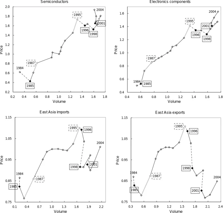
Given the heavy dependence of the East Asian countries on the electronics industry and substantial medium‐term fluctuations in the world electronics market, it is not surprising that the latter affect the economies of these countries. As an illustration, Figure 4 plots the price/quantity movements of world trade in semiconductor and other electronic components, together with those of the aggregate imports and exports of six Asian
countries.4 As semiconductors account for a sizable portion of international trade in
electronic parts and components, it is natural that the dynamics of the latter follows those of the former closely. More interesting is that their movements also seem to be reflected in the price/volume dynamics of the Asian countries’ aggregate trade. Although the plots in the lower panels may not look very similar to those of the upper panels, this is partly because the import and export prices of many countries collapsed in the wake of the Asian crisis. On closer examination, we find that the Asian countries’ import and export prices tended to
3 In Figure 3, the correlation between the growth rates of the global semiconductor shipment and the world GDP is 0.172 (1985‐1994) and 0.662 (1995‐2004) while that between the growth rates of the US electronics new orders and the real US GDP was 0.417 (1985‐1994) and 0.739 (1995‐2004). For 20 years between 1985 and 2004, the standard deviations of the annual growth rates of world chips shipments and US electronics orders were 17.6 and 9.7 percent,whereas those for the world and US GDP were 0.9 and 1.3 percent, respectively. 4 These countries include Hong Kong, Korea, Malaysia, Singapore, Taiwan and Thailand. Indonesia,
the Philippines and China are excluded due to the lack of appropriate official data (see Section 3). Data for Malaysia are lacking for some years.
make a upward excursion in years when there was a major hike in the world semiconductor price (e.g. 1987 and 1995) whereas the converse was the case when the latter fell sharply (e.g. 1985, 1996, 1998 and 2001). We also note that the import and export prices of the Asian countries tend to commove closely, reflecting their sensitivity to the cyclicality of the world electronics market and perhaps also indicating that most countries are price takers in both of the import and export markets. In what follows, we refer to these medium‐term fluctuations in the electronics market as the global electronics cycle (GEC) and investigate its relationship with the East Asian economies more closely. 3. TRADE COMPETITIVENESS BETWEEN CHINA AND OTHER ASIAN COUNTRIES In recent years, there has been lively debate about China’s increasing presence in regional and world trade and its implication for other East Asian countries. According to Fernald and Loungani (2004), there are at present two opposing views on this issue. In one view, China and other Asian countries as “comrades”, that is, China’s phenomenal export growth in recent years is largely or entirely benign to other Asian countries. Those who subscribe to this view point out that substantial parts f China’s exports are accounted for by foreign multinationals’ processing trade while the country’s growing economy provides a much‐needed new market for its neighbors (Kwan 2002; Weis 2004). The other view, in contrast, regards China and the other Asian countries primarily as competitors. Those who support this view typically stress increasing similarity of their export goods and China’s rising export share in third‐country markets, as well as its rising share in world inward foreign direct investment (Schott 2004; Kumakura 2005a). Not surprisingly, those who take the former view tend to be skeptical about the ability of exchange rates to adjust China’s external balance, whereas those who subscribe to the latter are often less so.
Those who question the view that China and other Asian countries are engaged in a fierce trade war often point out the fact that their exports tend to comove closely. Following Fernald and Loungani (2004), we plotted in Figure 5 the yearly growth rates of exports from
China and eight East Asian countries (ANIES4 + ASEAN4, henceforth abbreviated as EA8).5 Although China’s exports have recently grown much faster than those of EA8, we see that they do indeed tend to move in tandem.
Ahearne, Fernald, Loungani and Schindler (2003) note that the preceding visual impression can yet be deceptive, since the relationship between the exports of China and EA8 may be negative once their proximate determinants have been controlled for. To investigate this possibility, Ahearne et al. estimate the following regression model for the eight East Asian countries i = 1, 2, .., 8:
∆
x
i t,= +
α
∑
j=0β
j∆
f
i t,−j+
∑
k=0γ
k∆
s
i t k,−+
∑
l=0δ
l∆
x
CHN t l,−+ +
...
ε
i t, (1)
where
x
i t, denotes country i’s real exports in period t,f
i t, is the foreign income,s
i t, isthe real effective value of the currency of country i,
x
CHN t, is the real exports of China (all in natural logarithm), andε
i t, is the error term. In this and the next section, we write the rate of change in the real effective value of country i’s currency in each period as ∆si t, ≡∑
jω
j t,∆si j t/ , ≡∑
jω
j t,(
∆ei j t/ , + ∆pj t, − ∆pi t,)
(2)where
e
i j t/ , is the log of the price of one unit of country j’s currency in i’s currency),p
i t, isthe price level in country i, and
ω
j t, is the share of currency j in the effective exchange rateindex. Thus a positive value of
∆
s
i t, indicates currency i’s real depreciation.Ahearne et al.’s estimation results are reproduced in Table 3. They obtained these results by pooling the data for ANIES4, ASEAN4 and EA8 and estimated eq. (1) with the
fixed effect model.6 We observe that the coefficient on the contemporaneous Chinese export growth is positive in all cases and statistically significant at the 10 percent level for ASEAN4. 5 As a large portion of China’s exports is mediated by Hong Kong, we also show the growth rate of aggregate exports from China and Hong Kong (excluding their mutual trade), together with that of EA8 other than Hong Kong.
6 As the original article defines a rise in the real exchange rate as an appreciation of the home
Ahearne et al. note that these results are “inconsistent with most stories of severe, cutthroat competition between China and the rest of Asia” (Ahearne et al. 2003, pp.7). More recently, a team of economists at the Hong Kong Monetary Authorities have re‐estimated eq. (1) with updated data and using a few alternative estimation methods (Cutler, Chow, Chan and Li 2004). In their results, too, the estimates of
δ
l are generally positive and often statistically significant (Cutler et al. 2004, pp. 22).7The result in Table 3, however, contains a few puzzles. First, while the exports of China and other Asian countries may indeed be more complementary than commonly
believed, the coefficients on
∆
x
CHN t, are much larger for lower‐income ASEAN4 thatpresumably compete more directly with China in export markets, than for higher‐income
ANIES4. In addition, the estimated coefficients on the foreign income
∆
f
i t, are allextremely large, suggesting that the exports of the Asian countries have the income elasticity of 3.0‐5.2. Although Cutler et al.’s estimates of its coefficient are slightly smaller, they still range between 1.6 and 3.13.
As far as we can see, there are two problems in the foregoing estimation, and both of these problems are related closely to the global electronics cycle (GEC). The first and relatively straightforward problem is that eq. (1) does not take into account the effect of GEC on the exports of the Asian countries. As we saw in Section 2, electronics constitute the bulk of their exports, and the cycle of the global electronics industry has historically been correlated only partially with the world business cycle. Although Ahearne et al. (2003) do not explain how they computed
∆
f
i t, , Cutler et al. (2004) define this variable as the growth rate of the world real GDP excluding that of country i. Thus it seems likely that much of the impact of the GEC on the Asian countries’ exports is missed out in their estimation. The second and slightly more subtle problem concerns the way in which Ahearne et al.and Cutler et al. compute
∆
x
i t, and∆
x
CHN t, . Both authors merely state that these variablesare the growth rates of each country’s “real” exports and do not explain how the nominal export values are deflated. If we interpret eq. (1) as an export demand function, the most
suitable deflator is the export price index, preferably one constructed directly from customs data. As far as we know, however, the Chinese authorities provide no official export price index, and those for some other countries are missing as well. Our suspicion is that Ahearne
et al. and Cutler et al. compute
∆
x
i t, and∆
x
CHN t, either by deflating the nominallocal‐currency export values by the local‐currency CPI (or perhaps the GDP deflator), or by deflating the nominal US‐dollar exports by the US CPI. Although such deflation methods are quite common in cross‐country regressions, there are at least two reasons to suspect that they are problematic in our present setting. First, as many Asian countries’ exports are concentrated on electronics, the commodity composition of their exports must be very different from the commodity basket of their domestic price indices. Second, we saw in Figure 4 that the aggregate export price of the East Asian countries was correlated with the
GEC. This points to the possibility that not only do
∆
x
i t, and∆
x
CHN t, in Ahearne et al. andCutler et al. fail to track the actual export volume accurately but also suffer a systematic bias
arising from the GEC.8
8 Partly motivated by the result of Ahearne et al. (2003), Eichengreen, Rhee and Tong (2004) also
investigate export complementarity between China and other Asian countries. Rather than measuring the correlation between their aggregate exports, Eichengreen et al. estimate the following (modified) gravity model using annual bilateral trade data for 1990‐2002
xi,j,t ≡ a + b * xCHN,j,t + c * Zi,j,t + ei,j,t
where xi,j,t and xCHN,j,t are the real exports of, respectively, Asian country i and China to third country j, and Zi,j,t is a vector of standard gravity‐equation arguments. To control for unobserved factors that simultaneously influence xi,j,t and xCHN,j,t, Eichengreen et al. estimate this equation with two‐stage least squares (2SLS), first estimating an independent gravity equation for xCHN,j,t and then using its predicted value as an instrument for the foregoing regression model. In their baseline estimation, the estimated value of b is ‐0.18 with the standard error of 0.02.
As the above regression refers only to the exports to third countries, the estimated value of b is not directly comparable to δl in Ahearne et al. As China’s export share in major third markets has recently risen sharply, the positive correlation between the aggregate exports of China and other countries found by Ahearne et al. almost certainly reflects the growing imports of China from the latter countries. And as China’s import growth should be driven at least partly by its rising income level, and as its income is in turn correlated strongly with its exports, one cannot get the full picture unless one obtains the quantitative relationship among these three variables. Eichengreen et al. thus
Before investigating how much the results in Table 3 are influenced by these two problems, we first reestimate eq. (1) by making only minimum modifications to the relevant
variables. First, we generate the time series of
∆
f
i t, by taking a weighted average of thereal GDP growth rates of 26 foreign countries, where the weight is the (time‐varying) share of each foreign country in country i’s exports. As the Asian countries’ trade relations are not
homogeneous and have changed substantially over time, the series of
∆
f
i t, computed inthis way should capture more closely the external demand for each country’s exports. Second, although Ahearne et al. and Cutler et al. seem to use a CPI‐deflated real exchange
rate index for
∆
s
i t, , it is unlikely that CPI‐based effective exchange rates provide a goodmeasure of each country’s export competitiveness (Kumakura 2005a). We thus create for each country an original effective exchange rate index based on the PPI for the manufacturing or industrial sector, assuming that this index does a better job of tracking the local exporters’ production costs.9 And lastly, we compute , i t
x
∆
and∆
x
CHN t, by deflatingnominal local‐currency export values with the manufacturing PPI rather than the CPI, as the former’s volume weights should be closer to those of exports. See Appendix C for the data source and details on the construction of individual variables.
We estimate eq. (1) using updated annual data for 1985‐2004, taking into account the fact that China’s integration to the world economy in earlier years had been rather
estimate yet another gravity equation for Chinese imports and, by combining the estimated income elasticity of its imports with the preceding result, calculate the net impact of China’s 10 percent income growth on the exports of the other Asian countries. The computed full effect is positive for a few high‐income countries (e.g. Korea) but mildly negative for other East Asian countries (and more significantly so for most South Asian countries).
Thus the end result of Eichengreen et al. is less optimistic than those of Ahearne et al. and Cutler et al. One reason why the result we will find below is closer to that of Eichengreen et al. is that their 2SLS estimation controls (perhaps inadvertently) for the simultaneous impact of the GEC on the exports by China and the other countries. Eichengreen et al., however, compute xi,j,t and xCHN,j,t by deflating nominal US dollar export values by the US CPI, a method unlikely to provide an accurate proxy for the actual export volumes; see below.
9 For countries where a suitable PPI was unavailable, we used the WPI for export and
tenuous.10 As we shall discuss later, our series of , i t
x
∆
and∆
x
CHN t, in fact still fail to track properly changes in the genuine export volumes. In many countries affected badly by the Asian crisis, for example, the computed values of∆
x
i t, in 1998 tend to be implausibly large,most certainly reflecting the fact that their domestic PPI responded more slowly and by
smaller amounts to the collapse of the home currency than did their export prices.11 We
thus remove 1998 from our sample by adding a year dummy variable to eq. (1). We also eliminate the lagged dependent variable from the set of regressors, since lagged regressands can cause a serious estimation bias in panel regression, particularly when the time dimension of the data set is not very long (Judson and Owen 1999).
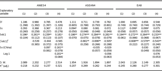
The result of our estimation is shown in Table 4. Despite the fact that we retained Ahearne et al.’s basic specification, our result differs substantially from theirs. First, the coefficient on China’s export growth is positive for ANIES4 but negative for ASEAN4, quite
opposite to their result. Second, although the coefficient on
∆
s
i t, remains positive andstatistically significant, their values are twice to three time larger than what we saw in Table 3. These observations suggest that the results reported by Ahearne et al./Cutler et al. are sensitive to the choice of the price index with which to compute export volume and real exchange rates. As we will see later, for many Asian countries even the PPI‐based effective exchange rate is in fact not a good measure of external competitiveness; we should not thus
put much trust in the large coefficients on
∆
s
i t, are in Table 4.Let us now examine the first of the two problems noted above. To test if the GEC really has an independent explanatory power for the export performance of the Asian countries, we modify Ahearne et al.’s regression model as follows:
∆
x
i t,= +
α
∑
j=0β
j∆
f
i t,−j+
∑
k=0γ
k∆
s
i t k,−+
∑
m=0φ
m∆
elc
t m−+ +
...
ε
i t, (3)
where
∆
elc
t m− is a variable that reflects the state of the world electronics market. While
10 Extending the sample to 1981, however, does not materially change the results that follow.
11 For example, the values of ∆xi, 1998 for Indonesia and Korea are 1.526 and 0.322 (i.e. increases in
there are a number of candidates for this variable, we saw in Section 2 that the cycle of the global electronics industry was typically accompanied by changes in both the prices and the volumes of relevant products, with no mechanical relationship between the two. This
suggests that we will miss much of the dynamics of the electronics industry if we let
∆
elc
i t, be represented solely by a price or quantity variable. By taking this point into account, we first consider the following indicator of the GEC:(
)
(
)
1, Global sales of semiconductor devices in nominal US dollars
World GDP in nominal US dollars
ln
ln
t t telc
∆
≡ ∆
− ∆
(4)where the global sales of semiconductors include both those shipped within individual countries and traded between two countries. While it is possible to interpret this variable as a “real” growth rate of the world semiconductor market, we consider it as representing the part of the cyclical fluctuations in the global electronics market that are not attributable to the world business cycle.12 If we let , elc t
p
∆
and∆
p
t denote the rate of change in the price of semiconductors and the world inflation rate (both measured in US dollars), and∆
y
elc t,and
∆
y
t the real growth rates of the volume of global semiconductor shipment and theworld GDP,
∆
elc
1,t can be written as
∆
elc
1,t= ∆
(
p
elc t,+ ∆
y
elc t,)
− ∆ + ∆
(
p
ty
t)
= ∆
(
p
elc t,− ∆
p
t) (
+ ∆
y
elc t,− ∆
y
t)
(5)
In general, therefore, our measure of GEC departs from 0 whenever the dynamics of the global semiconductor market deviates from those of the world economy on either or both of
the price and the quantity margins. The series of
∆
elc
1,t computed as above still turned out
12 Note that a downturn in the world electronics market can depress the exports of each Asian
country not only directly by reducing the amount of electronic goods it can sell in the international market but also indirectly by slowing down the economies of its export‐destination countries and depressing their import demand for other products. When eq. (3) is estimated with ∆elc1,t, most of
this latter effect should appear in the coefficient on ∆fi,t, even if its fundamental cause is a change in ∆elc1,t. Thus, if the coefficient on ∆elc1,t still turns out to be statistically significant, that would suggest
that GEC has an explanatory power for the exports of the Asian countries over and above its indirect effect through foreign income.
to be quite volatile over time. Thus we add the square of this variable to eq. (3) so as to allow for the possibility that its effect on the regressand is non‐linear.
The result of our estimation is in Table 5. This table omits the results for specifications
that include lagged explanatory variables (other than
∆
x
CHN t,−1) as most of their coefficientswere either statistically insignificant or had the unexpected sign. The term representing the
GEC is highly significant in all specifications, with some indication of nonlinearity.13 We
also notice that the estimated coefficients on
∆
f
i t, are substantially smaller than what wefound in Table 4, suggesting that our previous estimation confounded the effect of foreign
income with that of the GEC. In regressions for ANIES4, the coefficients on
∆
x
CHN t, are stillpositive but no longer statistically significant; in regressions for ASEAN4, its coefficient remains significant and even more negative than in Table 4. In general, our result seems to indicate that the GEC is an important determinant of the Asian countries’ exports.
In a few East Asian countries, however, semiconductors constitute a leading export
product. Although we are here interpreting
∆
elc
1,t not literally as the growth rate of worldsemiconductor sales but an indicator of the cyclical condition of the wider electronics
market, its value is in practice determined jointly with
∆
x
i t, . To the extent that this is thecase, there is legitimate concern about estimation bias due to the endogeneity between the regressand and our GEC variable. As a check on this possibility, we consider an alternative indicator of the GEC and see how using this variable affects the preceding result. Here we consider the following variable
(
)
(
)
2, New orders for electronic goods in the USA in nominal US dollars
USA GDP in nominal US dollars
ln
ln
t t telc
∆
≡ ∆
− ∆
(6)As the share of the United States in the world electronics consumption is very large, the growth rate of the new orders for electronic goods in the country is widely used as an indicator of the state of the world electronics market (see, for example, Ping et al. 2004). As
13 Although the estimated coefficients on ∆elc1,t are small compared to the coefficients on ∆fi,t, the
standard deviation of ∆elc1,t during the sample period is 0.173 while those of ∆fi,t ranges between 0.012 and 0.014.
the US new orders only concern those received by local manufacturers, estimating eq. (3) with this variable should help alleviate the potential endogeneity problem.
The result is shown in Table 6. As the square of
∆
elc
2,t was not statisticallysignificant,14 this table shows the results for specifications that include only the linear terms.
In general, the estimated coefficients of
∆
elc
2,t are large and statistically significant, andthe overall fit of the equation is comparable to Table 5. Although the coefficient on
∆
elc
2,tis only marginally significant for ANIES4, this is apparently due to fairly strong correlations
between
∆
elc
2,t with∆
f
i t, .15 This multicollinearity problem is reflected in the coefficientson
∆
f
i t, , whose estimates are larger than the corresponding values in Table 5. Otherwisethe results are similar to Table 5, including the sign and the value of the coefficient on
,
CHN t
x
∆
.16Let us now consider the second of the two problems mentioned earlier. As noted previously, China reports no official export price index while those for Indonesia, Malaysia
and the Philippines are either unavailable or available for only a limited period.17 We thus
first limit our attention to the five countries for which official unit export value indices are available (Hong Kong, Korea, Singapore, Taiwan and Thailand) and generate for each of
these countries an alternative series of
∆
x
i t, by taking the difference between the growthrates of its export values and unit value index. We then pool the data for the five countries
and estimate eq. (3), using alternatively the previous and the new series of
∆
x
i t, as the
14 This evidently reflects the fact that ∆elc2,t is less volatile than ∆elc1,t (see Figure 3).
15 ∆elc2,t has been correlated fairly tightly with the US business cycle in recent years whereas some of
ANIES4 (e.g. Korea and Taiwan) depend particularly heavily on the Untied States as their export market. In these countries, therefore, ∆elc2,t is inevitably correlated with ∆fi,t.
16 As yet another check on the potential simultaneity bias, we estimated eq. (3) using the values of ∆xi,t and ∆xCHN,t that are computed by excluding semiconductors (SITC 776) from each country’s total exports. The electronics variable still tuned out to be highly significant, suggesting that the impact of the GEC on the exports of the Asian countries extends well beyond the semiconductor sector itself.
17 Although Indonesia reports import and export price indices, these are based on survey data at the
dependent variable. As there is no new series for Chinese exports, we do not include
,
CHN t
x
∆
in this round of estimation.The result is shown in Table 7. As is immediately clear, the two sets of regressions generate very different results. First, when the dependent variable is the “proper” volume growth rate, the coefficients on the contemporaneous real exchange rate variable are
invariably small and are not estimated precisely. Second, although
∆
elc
1,t and∆
elc
2,tremain highly significant in both sets of regressions, the estimated coefficients are generally larger when the dependent variable is the volume growth rate. While the coefficients on the lagged electronics variables have the unexpected sign in all regressions, this appears to reflect high collinearity among the explanatory variables. All in all, Table 7 is a sobering reminder that at least for the countries under consideration, deflating nominal exports with domestic price indices is not a reliable way of approximating the actual export volume.
Strictly speaking, the unit export value indices used above are not comparable across the countries, since they are not compiled with the same formula and not all of them are based exclusively on customs statistics. Moreover, as many of these indices are a Laspeyres index with only periodic adjustments of the quantity weights, there may be some bias due
to changes in the composition of export commodities.18 Recently, a team of economists at
the Japanese Institute of Developing Economies (IDE) has compiled annual unit import and export value indices for a number of industrial and emerging Asian countries (Noda 2005). The IDE indices are based on detailed customs data gathered from either the UN COMTRADE or national sources and were subjected to extensive consistency tests, although the institute still continues its efforts to improve their reliability. The current versions of the indices are available in a number of alternative formats, including a chain‐linked Fischer index (CLFI) that is least likely to suffer from large measurement
errors.19 As a further check on our previous result, we recompute , i t
x
∆
and∆
x
CHN t, using 18 The Laspeyres export price index is prone to a bias when the same volume weights are used for a prolonged period. Barth and Dinmore (1999) provide a related discussion in the context of the Asian countries. 19 When a volume index is derived by dividing nominal values by a chain‐linked Fischer price index,this IDE‐CLFI and repeat the previous estimation for EA8. As our new series of
∆
x
i t, and ,CHN t
x
∆
exhibit no obvious anomalies during the Asian crisis, we drop this time the yeardummy for 1997. The sample period is 1986‐2003 due to the availability of the IDE price
index for China.20
The result of this last set of regressions is shown in Table 8. The coefficients on
∆
f
i t,now range between 0.5 and 1.2, which look more plausible than what we saw previously.
The coefficients on
∆
s
i t, are of the expected sign but, as in the right columns of Table 7,numerically small and only marginally significant. The coefficients on
∆
elc
1,t are generallysignificant and large, as are those on its square term. Lastly, the coefficients on
∆
x
CHN t, arepositive for ANIES4 but negative for ASEAN4 ‐‐‐ again similar to the previous regressions ‐‐‐ although they are now statistically insignificant in most cases. In the end, therefore, the
only variable that remained unambiguously significant throughout this section was those
pertaining to the electronics cycle.
Why, then, did using the export volume variable generate the regression results that are so different from those based on the PPI‐deflated “real” exports? To shed light on this question, we computed for each of EA8 and China the difference between the annual inflation rates of the domestic price indices (CPI or PPI) and the rate of nominal depreciation of the home currency against the dollar, for each year during our estimation period. If the local‐currency prices of export goods are synchronized closely with the general domestic price level, the calculated values should be a good proxy for the rate of change in the aggregate export price measured in US dollars. Figure 6 compares the time series of the computed values with the corresponding rate of change in the IDE‐CLFI, which is also measured in US dollars and should represent the actual export price movement with
reasonable accuracy.21 As we can see in the upper panel, however, the dollar‐converted CPI
the former also becomes a chain‐linked Fischer index.
20 The original IDE unit export value index for Hong Kong was compiled for the country’s total
exports including re‐exports. We thus requested the IDE staff to compile a new index for its domestic exports, from which the country’s volume growth rate was computed.
and PPI do not track the IDE index well, even excluding the period of the Asian crisis when the former completely undershot the latter. On closer examination, we also notice that the years in which the inflation rate of the IDE‐CLFI is visibly higher than those of the other two series ‐‐‐ 1987, 1889, 1995 2000, and 2003 ‐‐‐ all correspond to years when the price of
semiconductors shot up in the international market (see Figure 2).22
The foregoing observation suggests that if we compute
∆
x
i t, not from an explicitexport volume index but in terms of CPI‐ or PPI‐deflated “real” exports, its value is systematically biased upward when the international prices of electronic goods are rising faster than the domestic price level, which typically coincide with upturns in the electronics
cycle. As we saw before,
∆
f
i t, also tends to have a higher value when the world electronicsmarket is booming, as the latter is often boosted by a strong US economic growth and in turn tends to push up the growth rates of the Asian economies (see Section 4). Then if we regress the CPI‐ or PPI‐based “real” export growth rate on an equation like (1), we are
bound to find a large coefficient on
∆
f
i t, not only because this variable will inevitably pickup some of the effects attributable to the GEC but also because of its artificially inflated correlation with the dependent variable. This indeed seems to be one reason why we found
puzzlingly large values for the coefficients on
∆
f
i t, in Tables 3 through 7.The preceding analysis also points to the possibility that our measure of
∆
s
i t, doesvalues for the eight Asian countries, where the weight is the share of each country in their aggregate exports measured in US dollars.
22 In China, however, the GEC does not seem to have a systematic effect on the discrepancies
between the IDE unit value index and the two dollar‐converted domestic price indices (Figure 6, lower panel). We can think of a few reasons why this is the case. First, although electronics now constitute a sizable part of China’s exports, the share of electronic goods in its total exports started to surge only in mid‐1990s (Table 2). Second, China maintained until 1993 a dual exchange rate regime and a system of foreign exchange retention quotas, which should have driven a wedge between the exporters’ nominal sales and their effective revenues (Mehran et al. 1996). Third, China’s domestic prices have been liberalized in steps during the 1980s and 90s ‐‐ often engendering a bout of price hikes ‐‐ and should have been influenced heavily by factors unrelated to external development (Feyzioğlu 2004). At least during the last few years, however, the discrepancies between China’s export price index and two domestic price indices have been very similar to those for EA8.
not accurately represent each country’s export competitiveness. As we saw in Figure 3, the GEC seems to exert significant influence on both the export and import prices of the East Asian countries. As the electronics industries of many Asian countries rely heavily on imported components, a large increase in the international prices of the latter should add measurably to their production cost, of which only part is likely to be passed onto their export prices. To the extent that this is the case, a real exchange rate index computed with the domestic CPI or PPI can deviate from the external competitiveness of home producers not merely because a large exchange rate movement tends to drive a wedge between the domestic price level and the prices of traded goods, but also because it misses an important part of the systematic impact of the GEC on the profitability of the domestic electronics
producers.23 We will revisit this issue in the next section.
As it should to take time for China’s economic and export growth to have their full effect felt on its neighbors, whether China and the other emerging Asian countries are comrades or competitors is clearly a medium‐ to long‐term question. To the extent that this is the case, one ought to be cautious about drawing an answer to this question from time‐series regressions like eqs. (1) and (3). Moreover, since these regressions address the cyclical determinants of Chinese exports only indirectly, we are still unsure about the relative importance of the GEC and other factors as determinants of its trade dynamics. In Appendix A, we look more closely on China’s recent trade statistics and argue that it is not quite accurate to consider the country simply as an assembly house for foreign multinationals.
4. YEN‐DOLLAR EXCHANGE RATE AND BUSINESS CYCLES OF EAST ASIAN COUNTRIES
Another issue that recurs in the literature on macroeconomic dynamics and monetary
23 One complicating factor is that the electronics industries of a few (though not all) Asian countries
are dominated by foreign multinationals, which tend to engage in extensive intra‐firm trade in production materials and components. Thus the impact of the GEC on the profitability of local operations is likely to differ across the countries.
coordination in East Asia is the relationship between the yen/dollar exchange rate and the economies of Japan and other countries in the region. While the relative economic position of Japan, China and other Asian countries has changed dramatically during the past few decades, Japan still remains a major player in regional trade and an important provider of foreign direct investment (FDI). A number of authors argue, in particular, that recurrent swings in the yen/dollar exchange rate have been an important source of macroeconomic instability, not only in Japan but also among other Asian countries (McKinnon 2005).
Although one can conceive of a number of channels through which a large swing in the yen/dollar exchange rate might affect the emerging Asian economies, what is most stressed in the literature is its effect on their export performance. For example, Ito, Ogawa and Sasaki (1999) note that the export growth rates of emerging Asian countries are correlated negatively with the real exchange rates between their currencies and the yen, suggesting that the latter is responsible for the former. Similarly, McKinnon and Schnabl (2003) point out that the business cycles of these countries are correlated strongly with one another, and claim that their synchronized output cycles are generated principally by medium‐term fluctuations in the yen/dollar exchange rate. Corsetti et al. (1999) and Doraisami (2004) note the fact that the yen depreciated sharply vis‐à‐vis the dollar since mid‐1995 through 1998, during which the growth rates of most Asian countries’ export earnings have either decelerated markedly or ground to a halt. In their view, the post‐1995 yen depreciation was an important causal factor behind the subsequent Asian crises.
As one can see, the preceding views all rest on the assumption that most East Asian currencies are either pegged or kept stable vis‐à‐vis the US dollar, for otherwise there is little reason for nominal yen/dollar fluctuations to immediately change the relative export competitiveness between Japan and other Asian countries. And this is indeed the dominant view in the literature. The pre‐crisis exchange rate regimes of most Asian countries are widely described as de facto dollar pegs while some authors even argue that many crisis‐affected countries have recently revived their dollar peg policies (Fukuda 2002; McKinnon 2005). As these authors all recommend some kind of regional exchange rate arrangement as a means to enhancing macroeconomic stability in East Asia, the relationship between the yen/dollar exchange rate and the regional economies has implications for a
number of policy issues.
The existing literature provides several econometric “evidence” in support of the view that yen/dollar fluctuations constitute the principal macroeconomic destabilizer in East Asia. For example, Kwan (2001) and McKinnon and Schnabl (2003) test this hypothesis by estimating the following simple OLS model:
∆
y
EA t,= + ∆
α β
y
USA t,+ ∆
γ
0e
Y / $,t+ ∆
γ
1e
Y / $,t−1+
ε
t (7) where∆
y
EA t, denotes a weighted average of the yearly real GDP growth rates of the nine East Asian countries (EA8 and China),24 , USA ty
∆
is the real growth rate of the United States (a proxy for the export demand), and∆
e
Y / $,t is the rate of nominal depreciation of the yen vis‐à‐vis the dollar. Their results are reproduced in Table 9 as reference for our succeedingdiscussion. As one can see, the estimated coefficients on
∆
e
Y / $,t and∆
e
Y / $,t−1 are allnegative and statistically significant at standard levels, whereas the US growth rate indicates little bearing on the dependent variable. Similarly, Ito et al. (1999) regress the export growth rates of six Asian countries on the GDP growth rates of the Unites States and Japan and the real exchange rate of their currencies vis‐à‐vis the dollar and the yen, and find for most countries that a depreciation of the home currency against the yen has a positive and statistically significant effect on the dependent variable. Doraisami (2004) also investigates the factors behind Malaysia’s export slowdown during the lead‐up to the Asian crisis, employing a more sophisticated error correction model and using the nominal yen/dollar exchange rate as a proxy for the Malaysian Ringgit’s misalignment. She finds that the yen/dollar rate is relevant to both the long‐ and short‐run export performance of Malaysia, with the yen’s fall vis‐à‐vis the dollar systematically depressing its export earnings. At first look, these results appear to corroborate the view that a large yen depreciation depresses the exports of emerging Asia and causes its economic slowdown.
In our view, however, these studies entail a few important problems, which are – as in the last section – related to the presence of the GEC. In the remainder of this section, we will