$v$-Support Vector Machine as Conditional Value-at-Risk Minimization (Mathematical Programming in the 21st Century : Optimization Modeling and Algorithms)

$\nu$

-Support Vector Machine

as

Conditional Value-at-Risk Minimization

Akiko

Takeda

Department

_of

Administration

Engineering,

Keio University,

3-14-1

Hiyoshi, Kouhoku, Yokohama, Kanagawa 223-8522, Japan Email address: takeda@ae.keio.ac.jp

Abstract

The $\nu$-support vector classification ($\nu$-SVC) algorithm

was

shown to work well and provide

intuitive interpretations, e.g., the parameter $\nu$ roughly specifies the fraction ofsupport vectors.

Although$\nu$correspondstoafraction,it cannot take the entirerangebetween_$0$

and 1 inits original

form. Thisproblemwassettledbyanon-convexextensionof$\nu$-SVCand the extendedmethodwas experimentally showntogeneralize better thanoriginalv-SVC. However,itsgood generalization performance andconvergencepropertiesof theoptimization algorithm have not been studied yet.

In this paper, we provide newtheoretical insights into these issues and proposea novel $\nu$-SVC algorithmthat hasguaranteed generalization performance and convergenceproperties.

1

Introduction

Support _vector

_{classification}

(SVC) is oneof the most successful classification algorithms in modern machineleaming (Scholkopf&Smola, 2002). SVCfindsahyperplane that separates training samples

indifferentclasses with maximummargin (Boser etal., 1992). Themaximummarginhyperplane

was

shownto minimize

an

upper boundofthegeneralization

error

accordingtothe Vapnik-Chervonenkis

theory (Vapnik, 1995). Thus the generalization performance ofSVC is theoretically guaranteed.

SVC

was

extendedtobe abletodealwithnon-separabledata bytrading the margin sizewith the data separation

error

(Cortes&Vapnik, 1995). This soft-margin formulation is commonly referred

to

as

C-SVC sInce the trade-offis controlled by the parameter $C$

.

C-SVC

was

shown to work very

well in awide range ofreal-world applications (Sch\"olkopf&Smola, 2002).

An alternative formulation of the soft-margin idea is $\nu$-SVC (Sch\"olkopf et al., $2000$)–instead

of the parameter $C,$ $\nu$-SVC involves another trade-off parameter

$\nu$ that roughly specifies the

frac-tion of support vectors (or sparseness of the solution). Thus, the $\nu$-SVC formulation provides us

richerinterpretation thanthe original C-SVC formulation, whichwould be potentially useful in real

applications.

Since the parameter $\nu$ corresponds to affaction, it should be able to be chosen between $0$ and

1. However, it

was

shown that _{admissible values of} $\nu$

are

actually limited (Crisp&Burges, 2000;

Chang&Lin, 2001). To cope with this problem, Perez-Cruz et al. (2003) introduced the notionof

negative margins and proposed extended $\nu$-SVC ($E\nu$-SVC) which allows $\nu$ to take the entire range

between $0$ and 1. They also experimentally showed that the generalization

performance of$E\nu$-SVC

is often better than that oforiginal $\nu$-SVC. Thus the extension contributes not only to elucidating

the theoretical property of$\nu$-SVC, but also to improving its generalization performance.

However, there remain two open issues in $E\nu$-SVC. Thefirst issue is that the

reason

why ahigh generalizationperformance

can

be obtainedby$E\nu$-SVC

was

not completely explained yet. Thesecond issueisthat theoptimization probleminvolved in$E\nu$-SVC is

non-convex

andtheoretical convergence properties of the $E\nu$-SVC optimization algorithm have not been studied _yet. The purpose of_this

After reviewing existing SVC methods in Section 2, weelucidate the generalization performance

of $E\nu$-SVC in Section 3. We first show that the $F_{\lrcorner}^{\urcorner}\nu$-SVC formulation could be interpreted

as

min-imization of the conditional $value- at- 7\dot{n}sk(CVaR)$, which is often used in finance (Rockafellar

&

Uryasev, 2002; Gotoh&Takeda, 2005). Then wegive newgeneralization error boundsbased onthe

$CVaR$ risk

measure.

This theoretical resultjustifies the use of$E\nu$-SVC.

In Section 4, we address non-convexity of the $E\nu$-SVC optimization problem. We first give a

new

optimization algorithm that is guaranteed to converge to

one

of thelocal optima within

a

finite

numberof iterations. Based onthis improved algorithm, wefurther show that the global solutioncan

be actually obtained within finite iterations

even

though the optimization problem is

non-convex.

Finally, in Section 5, we give concluding remarks and future prospects. Proofs of all theorems

and lemmas are sketched in (Takeda&Sugiyama, 2008).

2

Support Vector Classification

In this section,

we

formulatetheclassification problem and brieflyreview support vector algorithms.

2.1 Classification Problem

Let us address the classification problem of learning a decision function $h$ from $\mathcal{X}$ $(\subset$ IR$n)$ to $\{\pm 1\}$

based on training samples $(x_{i}, y_{i})(i\in M :=\{1, \ldots, m\})$

.

We

assume

that the training samples

are

i.i.$d$

.

following the unknown probability distribution _{$P(x, y)$} on $\mathcal{X}\cross\{\pm 1\}$

.

The goal of the classification task is to obtain a classifier $h$ that minimizes the generalization

error (or the risk):

$R[h]$ $:= \int\frac{1}{2}|h(x)-y|dP(x, y)$,

which corresponds to the misclassification rate for

unseen

test samples.

Forthe sake of simplicity, wegenerally focus on linear classifiers, i.e.,

$h(x)=$ sign$((w, x\}+b)$, (1)

where $w(\in \mathbb{R}^{n})$ is a non-zero normal vector, $b$ ($\in$ IR) is a bias parameter, and sign$(\xi)=1$ if$\xi\geq 0$

and $-1$ otherwise.

Most of the discussions in this paper can be directly applicable to non-linear kernel classifiers (Sch\"olkopf

&Smola,

2002). Thus we may not lose generality by restricting ourselves to linear classifiers.

2.2 Support Vector Classification

The Vapnik-Chervonenkis theory (Vapnik, 1995) showed that a large margin classifier has a small

generalization error. Motivated by this theoretical result, Boseret al. (1992) developedan algorithm for finding the hyperplane $(w, b)$ with maximum margin:

$\min_{w,b}\frac{1}{2}\Vert w\Vert^{2}$ $s.t$

.

$y_{i}(\langle w, x_{i}\}+b)\geq 1,$ $i\in M$

.

(2)

This is called (hard-margin) support vectorclassification (SVC) and valid when thetrainingsamples

2.3 C-Support

Vector Classification

Cortes and Vapnik (1995) extended the SVC algorithm tonon-separable

cases

and proposed trading

the margin size with the data separation error (i.e., “soft-margin”):

$\min_{w,b,\xi}\frac{1}{2}\Vert w\Vert^{2}+C\sum_{i=1}^{m}\xi_{i}$

s.t. $y_{i}(\langle w, x_{i}\}+b)\geq 1-\xi_{i}$, $\xi_{i}\geq 0$,

where $C(>0)$ _{controls the trade-off. This formulation is usually referred to}

_as

_{C-SVC, and}

_was

shownto work very well in various real-world applications (Scholkopf&Smola, 2002).

2.4

$\nu$-Support

Vector Classiflcation

$\nu$-SVC is another formulationofsoft-margin SVC

(Sch\"olkopfet al., 2000):

$\min_{w,b,\xi_{\rho}},\frac{1}{2}\Vert w\Vert^{2}-\nu\rho+\frac{1}{m}\sum_{i=1}^{m}\xi_{i}$

$s.t$

.

$y_{i}(\langle w, x_{i}\}+b)\geq\rho-\xi_{i}$, $\xi_{i}\geq 0$, $\rho\geq 0$,

where $\nu(\in m)$ is the trade-offparameter.

Sch\"olkopf et al. (2000) showed that if the $\nu$-SVC solution yields _$\rho>0$, C-SVC with$C=1/(m\rho)$

produces the

same

solution. Thus$\nu$-SVCandC-SVC

are

equivalent. However, $\nu$-SVChasadditional

intuitiveinterpretations, e.g., $\nu$is

an

upperbound

on

the fractionofmargin

errors

and

a

lowerbound

on

the fraction of support vectors (i.e., sparseness of the solution). Thus, the v-SVC formulation

would be potentially

more

useful than the C-SVC formulationin real applications.

2.5

$E\nu$

-SVC

Although $\nu$ has an interpretation

as

afraction, it cannot always take its fullrange between_$0$ and 1

(Crisp&Burges, 2000; Chang&Lin, 2001).

2.5.1 Admissible Range of$\nu$

For

an

optimal solution $\{\alpha_{i}^{C}\}_{i=1}^{m}$ ofdual C-SVC, let

$\zeta(C):=\frac{1}{Cm}\sum_{i=1}^{m}\alpha_{i}^{C}$,

$\nu_{\min}$ _{$:= \lim_{Carrow\infty}\zeta(C)$} and $\nu_{\max}$ $:= \lim_{Carrow 0}\zeta(C)$

.

Then, Chang and Lin (2001) showed that for $\nu\in(\nu_{\min}, \nu_{\max}]$, the optimal solution set of$\nu$-SVC is

the

same as

that ofC-SVC with some$C$ (not necessarily unique). In addition, the optimalobjective

valueof$\nu$-SVC is strictlynegative. However, for _{$\nu\in(\nu_{\max}, 1],$} $\nu$-SVCis unbounded, i.e., thereexists

no

solution; for$\nu\in[0, \nu_{\min}],$ $\nu$-SVCis feasiblewith

zero

optimalobjectivevalue, i.e.,

we

endup with

2.5.2 Increasing Upper Admissible Range

It

was

shown by Crispand Burges (2000) that

$\nu_{\max}=2\min(m_{+}, m_{-})/m$,

where$m+$ and$m$

-are

the number of positive and negative trainingsamples. Thus,whenthetraining

samples

are

balanced $(i.e., m+=m_{-}),$ $\nu_{ma)(}=1$ and therefore $\nu$

can

reach its upper limit 1. When

the training samples

are

imbalanced $(i.e., m+\neq m_{-})$, Perez-Cruz et al. (2003) proposed modifying

the optimization problem of$\nu$-SVC

as

$\min_{w,b,\xi_{\rho}},\frac{1}{2}\Vert w\Vert^{2}-\nu\rho+\frac{1}{m+}\sum_{i:y_{i}=1}\xi_{i}+\frac{1}{m_{-}}\sum_{i:y:=-1}\xi_{i}$

s.t. $y_{i}((w, x_{i}\}+b)\geq\rho-\xi_{i},$ $\xi_{i}\geq 0$, $\rho\geq 0$,

i.e., the effect of positive and negative samples

are

balanced. Under this modified formulation,

$\nu_{\max}=1$ holds

even

when training samples

are

imbalanced.

For the sake of simplicity, we assume $m+=m_{-}$ in the rest ofthis paper; when $m_{+}\neq m_{-}$, all

the results

can

besimplyextended in

a

similar way

as

above.

2.5.3 Decreasing Lower Admissible Range

When $\nu\in[0, \nu_{\min}],$ $\nu$-SVC produces

a

trivial solution $(w=0$ and $b=0)$

as

shown in Chang and

$L$in _$(2(K)1)$

.

To prevent this, Perez-Cruz et al. (2003) proposed allowing themargin

$\rho$ tobe negative

and enforcing the

norm

of$w$ to be unity:

$\min_{w,b,\xi_{\rho}},-\nu\rho+\frac{1}{m}\sum_{i=1}^{m}\xi_{i}$

s.t. $y_{i}(\{w,$ $x_{i}\rangle+b)\geq\rho-\xi_{i},$ $\xi_{i}\geq 0,$ $\Vert w||^{2}=1$. (3)

By this modification,

a

non-trivial solution

can

be obtained

even

for $\nu\in[0, \nu_{\min}]$

.

This modified

formulation is called extended $\nu$-SVC ($E\nu$-SVC).

The$E\nu$-SVCoptimization problem is

non-convex

dueto the equality constraint $\Vert w\Vert^{2}=1$

.

Perez-Cruz et al. (2003) proposed the following iterative algorithm for computing

a

solution. First, for some initial it, solve the problem (3) with $\Vert w\Vert^{2}=1$ replaced by $\{\tilde{w}, w\}=1$

.

Then, using the

optimal solution $\hat{w}$, update $\tilde{w}$ by

$\tilde{w}arrow\gamma\tilde{w}+(1-\gamma)\hat{w}$ (4)

for $\gamma=9/10$, and iterate this procedure until convergence.

Perez-Cruz et al. (2003) experimentally showed that the generalization performance of$E\nu$-SVC with$\nu\in[0, \nu_{\min}]$ isoftenbetterthan that with$\nu\in(\nu_{\min}, \nu_{\max}]$, implying that$E\nu$-SVCisapromising

classification algorithm. However, it is not clear how the notion of negative margins influences

on

the generalization performance and how fast the above iterative algorithm converges. The goal of

this paper is togive

new

theoretical insights into theseissues.

3

Justification of the

$E\nu$

-SVC

Criterion

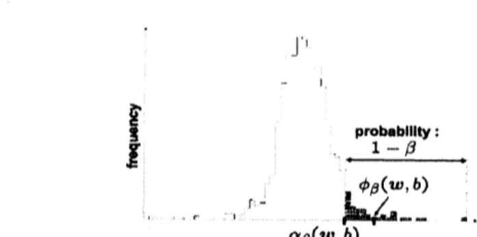
$\rfloor^{1}$ $-$ $\zeta\ovalbox{\tt\small REJECT}$ $\underline{pr_{1-\beta}obab|Ilty:}$ $\phi_{\beta}(w,b)$ $-rarrow$ $-R_{-}.,.$ , $d$

.

$\alpha_{\beta}(w,b)$

Figure 1: An example of the distribution of margin

errors

$f(w, b;x_{i}, y_{i})$

over

all training samples.

$\alpha_{\beta}(w, b)$ is the $100\beta$-percentile called the value-at-risk _$(VaR)$, and the

mean

_{$\phi_{\beta}(w, b)$ of the}

$\beta$-tail

distribution is called theconditional $VaR(CVaR)$

.

3.1

New Interpretation of

$E\nu$

-SVC

as

_$CVaR$

minimization

Let $f(w, b;x, y)$ _{be the margin}

_error

_{for a sample} $(x, y)$:

$f(w, b;x, y):=- \frac{y((w,x\rangle+b)}{||w||}$

.

Let

us

consider thedistribution of margin

errors

over

all training samples:

$\Phi(\alpha|w, b):=P\{(x_{i}, y_{i})|f(w, b;x_{i}, y_{i})\leq\alpha\}$

.

For $\beta\in[0,1)$, let $\alpha_{\beta}(w, b)$ be the _$100\beta$-percentile of the margin

error

distribution:

$\alpha_{\beta}(w, b):=\min\{\alpha|\Phi(\alpha|w,b)\geq\beta\}$

.

Thus only the fraction $(1-\beta)$ of themargin

error

$f(w, b;x_{i},y_{*}\cdot)$ exceeds thethreshold $\alpha\rho(w, b)$ (see

Figure 1). $\alpha_{\beta}(w, b)$is commonlyreferred to

as

thevalue-at-risk_$(VaR)$ in

finance and is often usedby

security houses

or

investment banks to

measure

the market risk of their asset portfolios (Rockafellar

&Uryasev,

2002; _{Gotoh&Takeda,} 2005).

Let

us

consider the $\beta$-tail distribution of_{$f(w, b;x_{i}, y_{i})$}:

$\Phi_{\beta}(\alpha|w, b):=\{$$\frac{0\Phi(\alpha|w,b)-\beta}{1-\beta}$

for$\alpha\geq\alpha_{\beta}(w, b)$

.

for $\alpha<\alpha_{\beta}(w, b)$,

Let $\phi_{\beta}(w, b)$ be the

mean

of the $\beta$-tail distribution of$f(w, b;x_{i},y_{i})$ (see Figure 1 again):

$\phi_{\beta}(w,b):=E_{\Phi_{\beta}}[f(w, b;x_{i}, y_{i})]$,

where $E_{\Phi_{\beta}}$ denotes theexpectationover the distribution $\Phi_{\beta}$

.

$\phi_{\beta}(w, b)$ is called the conditional _$VaR$

$(CVaR)$

.

_{By definition, the} $CVaR$_{is always larger than} or _{equalto the} $VaR$:

$\phi_{\beta}(w, b)\geq\alpha_{\beta}(w,b)$

.

(5)

Let usconsider the problem of minimizingthe $CVaR\phi_{\beta}(w, b)$ (which

we

referto

as

minCVaR):

$\min\phi_{\beta}(w,b)$

.

(6)

$w,b$

Figure 2: A profile of the $CVaR\phi_{1-\nu}(w^{*}, b^{*})$

as a

function of$\nu$

.

As shown in Section 4, the $E\nu-$

SVC optimization problem

can

be cast

as

a

convex

problem if $\nu\in(\overline{\nu}, \nu_{\max}]$, while it is essentially

non-convex

if$\nu\in(0, \overline{\nu})$

.

Theorem 1 The solution

_of

the $minCVaR$ problem (6) is equivalent to the solution

_of

the Ev-SVC

problem (3) urth

$\nu=1-\beta$

.

Theorem 1 showsthat $E\nu$-SVC actually minimizes the_{$CVaR\phi_{1-\nu}(w, b)$}

.

Thus,$E\nu$-SVCcouldbe

interpreted

as

minimizing the

mean

margin error over a set of “bad” training samples. In contrast, the hard-margin SVC problem (2)

can

beequivalently expressed in termsof the margin error

as

min

max

$f(w, b;x_{i},y_{i})$

.

$W,bi\in M$

Thus hard-margin SVC minimizes the margin

error

of the single ”worst” training sample. This

analysisshows that$E\nu$-SVC

can

beregarded

as an

extensionof hard-margin SVC to beless sensitive

to

an

outlier (i.e., the single ”worst” training sample).

3.2

Justification

of $E\nu$

-SVC

We have shown the equivalenoe between$E\nu$-SVC and minCVaR. Here

we

derive

new

bounds of the

generalization error based onthe notion of$CVaR$_{and tryto justify the} use _of$E\nu$-SVC.

When training samples

are

linearly separable, the margin

error

$f(w, b;x_{i}, y_{i})$ is negative for all

samples. Then, at the optimal solution $(w^{*}, b^{*})$, the$CVaR\phi_{1-\nu}(w^{*}, b^{*})$ is always negative. However,

in non-separable cases, $\phi_{1-\nu}(w^{*}, b^{*})$ could be positive particularly when $\nu$ is close to $0$

.

Regarding

the $CVaR$, we_{have the following lemma.}

Lemma 2 $\phi_{1-\nu}(w^{*}, b^{*})$ is continuousurith respect to$\nu$ and is strictly decreasing when$\nu$ is increased.

Let i7be such that

$\phi_{1-\overline{\nu}}(w^{*}, b^{*})=0$

if such $\overline{\nu}$ exists; we set _{$\overline{\nu}=\nu_{\max}$} if$\phi_{1-\nu}(w^{*}, b^{*})>0$ for all $\nu$ and we set $\overline{\nu}=0$ if_{$\phi_{1-\nu}(w^{*}, b^{*})<0$}

for all $\nu$

.

Then we have the following relation (see Figure 2):

$\phi_{1-\nu}(w^{*}, b^{*})<0$ for $\nu\in(\overline{\nu}, \nu_{\max}]$,

$\phi_{1-\nu}(w^{*},b^{*})>0$ for $\nu\in(0,\overline{\nu})$

.

3.2.1 Justiflcation When $\nu\in(\overline{\nu},$$\nu_{\max}]$

Theorem 3 Let $\nu\in(\overline{\nu}, \nu_{\max}]$

.

Suppose that support $\mathcal{X}$ is in a ball

of

radius _$R$ around the

$or\dot{\tau}gin$

.

Then,

_for

all $(w, b)$ such that $\Vert w\Vert=1$ and $\phi_{1-\nu}(w, b)<0$, there exists

a

positive constant $c$ such

that thefollowing bound hold with probability at least $1-\delta$:

$R[h]\leq\nu+G(\alpha_{1-\nu}(w, b))$, ₍₇₎

where

$G(\gamma)=\sqrt{\frac{2}{m}(\frac{4c^{2}(R^{2}+1)^{2}}{\gamma^{2}}\log_{2}(2m)-1+\log\frac{2}{\delta})}$

.

The generalization

error

bound in (7) is

_furthermore

upper-bounded

as

$\nu+G(\alpha_{1-\nu}(w,b))\leq\nu+G(\phi_{1-\nu}(w,b))$

.

$G(\gamma)$ ismonotone decreasing

as

$|\gamma|$increases. Thus,the above theorem showsthat when

$\phi_{1-\nu}(w, b)<$

$0$, the upper bound_{$\nu+G(\phi_{1-\nu}(w, b))$} is lowered ifthe

$CVaR\phi_{1-\nu}(w, b)$ is reduced. Since $E\nu$-SVC

minimizes$\phi_{1-\nu}(w, b)$ (see Theorem 1), theupper bound of thegeneralization

error

is also minimized.

3.2.2 Justification When $\nu\in(0, \overline{\nu}]$

Our discussion below depends

on

thesign of$\alpha_{1-\nu}(w, b)$

.

When$\alpha_{1-\nu}(w, b)<0$, we have the following

theorem.

Theorem 4 Let $\nu\in(0,\overline{\nu}]$

.

Then,

for

all $(w, b)$ such that $\Vert w\Vert=1$ and$\alpha_{1-\nu}(w, b)<0$, there exists

a positive constant$c$ such that the folloutng bound holds with probability at least $1-\delta$:

$R[h]\leq\nu+G(\alpha_{1-\nu}(w, b))$

.

The proof follows a similar line to the proof of Theorem 3. This theorem shows that when

$\alpha_{1-\nu}(w, b)<0$, theupper bound$\nu+G(\alpha_{1-\nu}(w, b))$ islowered if$\alpha_{1-\nu}(w, b)$ isreduced. Onthe other

hand, Eq.(5) shows that the $VaR\alpha_{1-\nu}(w, b)$ is upper-bounded by the _{$CVaR\phi_{1-\nu}(w, b)$}

.

Therefore,

minimizing $\phi_{1-\nu}(w, b)$ by $E\nu$-SVC may have

an

effect of lowering the upper bound of the

general-ization

error.

When $\alpha_{1-\nu}(w, b)>0$, wehave the following theorem.

Theorem 5 Let $\nu\in(0, \overline{\nu}]$

.

Then,

for

all $(w, b)$ such that $\Vert w\Vert=1$ and $\alpha_{1-\nu}(w, b)>0$, there exists

a positive constant$c$ such that the following bound hold with probability at least $1-\delta$:

$R[h]\geq\nu-G(\alpha_{1-\nu}(w, b))$

.

Moreover, the lower bound

_of

$R[h]$ is bounded

from

_above as

$\nu-G(\alpha_{1-\nu}(w, b))\leq\nu-G(\phi_{1-\nu}(w, b))$

.

The proof resembles to the proof ofTheorem 3. Theorem 5 implies that the lower bound $\nu-$

$G(\alpha_{1-\nu}(w, b))$ of the generalization

error

is upper-bounded by _{$\nu-G(\phi_{1-\nu}(w, b))$}

.

On the other

hand, Eq.(5) and $\alpha_{1-\nu}(w, b)>0$ yields $\phi_{1-\nu}(w, b)>0$

.

Thus minimizing $\phi_{1-\nu}(w, b)$ by $E\nu$-SVC

4

New optimization Algorithm

As reviewed in Section 2.5, $E\nu$-SVC involves a non-convex optimization problem. In this section,

we give

a new

efficient optimization procedure for $E\nu$-SVC. Our proposed procedure involves two

optimization algorithms depending

on

the valueof $\nu$

.

We first describe the two algorithms and then

show how these two algorithms

are

chosen for practical

use.

4.1

optimization

When $\nu\in(\overline{\nu}, \nu_{\max}]$

Lemma 6 When $\nu\in(\overline{\nu}, \nu_{\max}]$, the $E\nu- SVC$problem (3) is equivalent to

$\min_{w,b,\xi_{\beta}},-\nu\rho+\frac{1}{m}\sum_{i=1}^{m}\xi_{i}$

$s.t$

.

$y_{i}(\langle w, x_{i}\}+b)\geq\rho-\xi_{i},$ $\xi_{i}\geq 0,$ $\Vert w\Vert^{2}\leq 1$

.

(8)

This lemma shows that the equality constraint $\Vert w\Vert^{2}=1$ in the original problem (3)

can

be

replaced by $\Vert w\Vert^{2}\leq 1$ without changing the solution. Due to the convexity of $\Vert w\Vert^{2}\leq 1$, the above

optimization problem is

convex

and therefore

we

can

easily obtain the global solution oy

a

standard

optimization software.

4.2

optimization

When

$\nu\in(0, \overline{\nu}]$

If $\nu\in(0, \overline{\nu}]$, the $E\nu$-SVC optimization problem is essentially non-convex and therefore we need a

more

elaborate algorithm.

4.2.1 Local Optimum Search

Here, wepropose the following iterative algorithm for finding

a

local optimum. Algorithm 7 (The $E\nu$-SVC local optimum search algorithm for _{$\nu\in(0, \nu)$}

Step 1: Initialize $\tilde{w}$

.

Step 2: Solve the following linear

program:

$\min_{w,b,\xi,\rho}-\nu\rho+\frac{1}{m}\sum_{i=1}^{m}\xi_{i}$ (9)

s.t. $y_{i}(\{w,$ $x_{i}\rangle+b)\geq\rho-\xi_{i},$ $\xi\iota\geq 0,$ $\langle\tilde{w},$_$w\rangle=1$,

and let the optimal solution be $(\hat{w},\hat{b},\hat{\xi},\hat{\rho})$

.

Step 3: If$\overline{w}=\hat{w}$, terminate and output $\tilde{w}$

.

Otherwise, update $\tilde{w}$ by

$\tilde{w}arrow\hat{w}/||\hat{w}\Vert$

.

Step 4: Repeat Steps 2-3.

The linear program (9) is the

same as

the

one

proposed by Perez-Cruz et al. (2003), i.e., the

equalityconstrained $\Vert w\Vert^{2}=1$ of theoriginal problem (3) is replaced by $\langle\tilde{w},$$w\rangle=1$

.

The updating

ruleofth in Step 3 is different from the

one

proposed by Perez-Cruz et al. (2003) (cf. Eq(4)).

We define a “corner” (or “Odimensional face”) of $E\nu$-SVC (3)

as

the intersection of

an

edge of

the polyhedral cone formed by linear constraints of(3) and $\Vert w||^{2}=1$

.

Under the new update rule,

the algorithm visits

a corner

of$E\nu$-SVC (3) ineach iteration. Since $E\nu$-SVC has finite corners,

we

can

show that Algorithm7 with thenew updaterule terminates in afinite numberofiterations, i.e.,

Theorem 8 Algorithm 7terminates within a

_finite

number

_of

iterations

_of

Steps 2-3. $Fh$rthermore,

a solution

_of

the

_modified

$E\nu- SVC$algorithm is

a

_{local minimizer}

_if

_{it is unique and non-degenerate.}

4.2.2 Global Optimum Search

Next,

we

show that the global solution can be actually obtained within finite iterations, despite the

non-convexity of the optimization problem.

A naiveapproachto searching for theglobal _{solution is torunthe localoptimumsearch algorithm}

many times with different initial values and choose the best local solution. However, there is no

guarantee that this naive approach

can

find the global solution. Below,

we

givea

more

systematic

way to find the global solution based

on

the following lemma.

Lemma 9 When $\nu\in(0, \overline{\nu}]$, the Ev-SVCproblem (3) is equivalent to

$\min_{w,b,\xi,\rho}-\nu\rho+\frac{1}{m}\sum_{i=1}^{m}\xi_{i}$

s.t. $y_{i}((w, x_{i}\rangle+b)\geq\rho-\xi_{i},$ $\xi_{i}\geq 0,$ $||w\Vert^{2}\geq 1$

.

(10)

Lemma 9 could be proved in

a

similar way

as

Lemma 6. This lemma shows that the equality

constraint $||w||^{2}=1$ in the original Ev-SVC _{problem (3)}

can

_{be replaced by} $\Vert w\Vert^{2}\geq 1$ without

changing thesolution if$\nu\in(0,\overline{\nu}]$

.

Theproblem (10) iscalled

a

linear

reverse convex

prvgram (LRCP), whichis

a

class of

non-convex

problems consisting oflinear constraints and one

concave

inequality ($\Vert w\Vert^{2}\geq 1$ in the current case).

The feasible set ofthe problem (10) consists ofafinite number of

_faces.

For LRCPs, Horst and Tuy

(1995) showed that the local optimalsolutions correspond to 0-dimensional faces (or corners). This implies that all the local optimal solutions of the $E\nu$-SVC problem (10)

can

be traced by checking all the faces.

Let $D$ be the feasible set of$E\nu$-SVC (3). Below, we summarize the $E\nu$-SVC training algorithm

based

on

the cuttingplane method, which is

an

efficient method oftracing faces.

If the local solution obtained in Step 2 is

a comer

of $D$ (i.e., the local solution is not

on

any

cutting plane

as

(a) in Figure 3),

a

concavity cut (Horst&Tuy, 1995) is constructed. The concavity

cut has

a

roleof removing the local solution, i.e.,

a

0-dimensional face of$D$ and its neighborhood.

Otherwise,

a

_facial

cut (Majthay&Whinston, 1974) is constructed_{to eliminate the proper face} (see

(b) in Figure3).

Since the total number of distinct faces of$D$ is finitein the current setting and

a

facial cut

or a

concavity cut eliminates at least

one

faceat

a

time, Algorithm 10is guaranteed to terminate within

finite iterations (precisely, less than

or

equal to the number of all dimensional faces of $E\nu$-SVC).

which

are

better than the best local solution found

so

far, Algorithm 10 is guaranteed to trace

all

_sufficient

local solutions. Thus we

can

always find a global solution within finite iterations by

Algorithm 10. A more detailed discussiononthe concavity cut and the facial cut is shown in Horst

and Tuy (1995) and Majthay and Whinston (1974), respectively.

4.3

Choice

of Two

Algorithms

We have two convergent algorithms when $\nu\in(\overline{\nu}, \nu_{\max}]$ and $\nu\in(0,\overline{\nu}]$

.

Thus, choosing a suitable

algorithm depending

on

the value of $\nu$ would be

an

ideal procedure. However, the value of the

threshold V is difficult to explicitly compute since it is defined via the optimal value $\phi_{1-\overline{\nu}}(w^{*}, b^{*})$

(see Figure 2). Therefore, it is not straightforward tochoose

a

suitable algorithm for

a

given $\nu$

.

When we

use

$E\nu$-SVC in practice,

we

usually compute the solutions for several different values

of $\nu$ and choose the most promising

one

based on, e.g., cross-validation. In such scenarios,

we can

properly switch two algorithms without explicitly knowing the value of$\overline{\nu}$

–our

key idea is that the

solution of the problem (8) is non-trivial $(i.e., w\neq 0)$ if and only if $\nu\in(\overline{\nu}, \nu_{\max}]$

.

Thus if the

solutions

are

computed from large $\nu$ to small $\nu$, the switching point

can

be identified by checking

the trivialityof the solution. The proposed algorithm is summarized

as

follows.

Algorithm 11 (The $E\nu$-SVC algorithm for $(\nu_{\max}\geq)\nu_{1}>\nu 2>\cdots>\nu_{k}>0$)

Step 1: $iarrow 1$

.

Step 2: Compute $(w^{r}, b^{*})$ for $\nu_{i}$ by solving (8).

Step $3a$: If$w^{*}\neq 0$, accept $(w^{*}, b^{*})$

as

the solution for $\nu_{i}$, increment $i$, and go to Step 2.

Step $3b$: If $w^{*}=0$, _reject $(w^{*}, b^{*})$

.

Step 4: Compute $(w^{*}, b^{*})$ for $\nu_{i}$ by Algorithm 10.

Step 5: Accept $(w^{*}, b^{*})$

as

the solution for $\nu_{i}$, increment $i$, and go to Step 4 unless $i>k$

.

5

Conclusions

Wecharacterizedthe generalization errorof$E\nu$-SVCintermsof the conditional value-at-risk $(CVaR$,

see Figure 1) and showed that agood generalization performance is expected by $E\nu$-SVC. We then

derived

a

globallyconvergentoptimization algorithm

even

thoughtheoptimization probleminvolved

in $E\nu$-SVC is

non-convex.

We introduced the threshold $\overline{\nu}$based

on

thesign of the$CVaR$ (see Figure 2). We

can

check that

the problem (8) isequivalent to v-SVC in thesensethat they share thesamenegativeoptimal value in $(\overline{\nu}, \nu_{\max}]$ and $(\nu_{\min}, \nu_{\max}]$, respectively (Gotoh&Takeda, 2005). Onthe other hand, the problem (8) and $\nu$-SVC have the zero optimal value in $(0, \overline{\nu}]$ and _{$[0, \nu_{\min}]$}, respectively. Thus, although the

definitions ofVand$\nu_{\min}$

are

different, they would beessentially the

same.

We$wIl1$studythe relation

between $\overline{\nu}$and

$\nu_{\min}$ in more detail in the future work.

References

Boser,B. E.,Guyon, I. M.,&Vapnik, V. N. (1992). Atraining algorithmforoptimalmarginclassifiers. COLT

(pp. 144-152). ACM Press.

Chang, C.-C., &Lin, C.-J. (2001). Training $\nu$-support vector classifiers: Theory and algorithms. Neural Computation, 13, 2119-2147.

Cortes, C., &Vapnik, V. (1995). Support-vector networks. Machine Leaming, 20,273-297.

Crisp, D. J., &Burges, C. J. C. (2000). A geometric interpretation of$\nu$-SVM classifiers. NIPS 12 (pp. 244-250). MIT Press.

Gotoh, J., &Takeda, A. (2005). A linear classification model based on conditionalgeometric

score.

Pacific

Joumal

_of

optimization, 1, 277-296.

Horst, R.,&Tuy, H. (1995). Global optimization: Deterministic approaches. Berlin: Springer-Verlag.

Majthay, A., &Whinston, A. (1974). Quasi-concave minimization subject to linear constraints. Discrete

Mathematics, 9,35-59.

Perez-Cmz, F., Weston, J., Hermann, D. J. L., &Scholkopf, B. (2003). Extension ofthe $\nu$-SVM range

for classification. Advances in Leaming Theory: Methods, Models and Applications 190 (pp. 179-196).

Amsterdam: IOS Press.

Rockafellar, R. T., &Uryasev, S. (2002). Conditional value-at-risk for general loss distributions. Joumal

_of

Banking EYFinance, 26, 1443-1472.

Scholkopf, B., Smola, A., Williamson, R., &Bartlett, P. (2000). New support vector algorithms, Neural

Computation, 12, 1207-1245.

Sch\"olkopf, B., &Smola,A. J. (2002). Leaming with kernds. Cambridge, MA: MIT Press.

Takeda, A., &Sugiyama, M. (2008). $\nu$-Support Vector Machine as Conditional Value-at-Risk Minimization.

Proceedingsof the 25th Intemational Conferenceon Machine Leaming (ICML 2008), Helsinki, Finland.