ON HYPERBOLIC POLYNOMIAL DIFFEOMORPHISMS OF $\mathbb{C}^2$(New Trends and Applications of Complex Asymptotic Analysis : around dynamical systems, summability, continued fractions)

ON HYPERBOLIC POLYNOMIAL DIFFEOMORPHISMS OF $\mathbb{C}^{2}$

石井 豊 (九州大学数理学研究院)

YutakaISHII (Department ofMathematics, Kyushu University)

CONTENTS

1.

Introduction

and Main Result 1

2. Hyperbolicity: A Motivation 2

3. Some Preliminary Results ₂

4. A Criterion for Hyperbolicity ₃

5. Fusion ofTwo Polynomials 6

6. Rigorous Numerics Technique

₇

7.

Proof

of

Main Theorem

8

References ₉

1.

INTRODUCTION

AND MAIN RESULT

The purpose ofthis note is tosketch

a

proofof the result stated inMain Theorem below. Consider a cubic complex H\’enon map:

$f_{a,b}$ : (x,$y)\mapsto(-x^{3}+a-by,$x)

with $(a, b)=(-1.35,0.2)$ and let $J$ be the Julia set of $f_{a,b}$.

Main Theorem. The cubic complexH\’enon map above is hyperbolic but is nottopologically conjugate

on

$J$ to a small perturbation

of

any expanding polynomial in

one

variable.

Here, a H\’enon map or, more generally, a polynomial diffeomorphism $f$ of $\mathbb{C}^{2}$ is said to

be hyperbolic if its Julia set is

a

hyperbolic set for $f$ (see Definition 2.2 and Lemma 3.3). Hyperbolic polynomial diffeomorphismsof$\mathbb{C}^{2}$

have beenextensively studied, e.g., from the

viewpoint of Axiom A theory by [BS1] and the combinatorial point of view \‘a _la

Douady-Hubbard by [BS7]. In $[\mathrm{H}\mathrm{O}2, \mathrm{F}\mathrm{S}]$ it has been shown that a sufficiently small perturbation

of any expanding polynomial$p(x)$ ofone variable in the generalized H\’enonfamily: $f_{p,b}$ : $(x, y)\mapsto(p(x)-by, x)$

is hyperbolic. However, this

was

sofar the only known example of

a

polynomial diffeomor-phism of$\mathbb{C}^{2}$ which

was

rigorouslyshown to be hyperbolic. Moreover, the dynamics

ofsuch

$f_{\mathrm{p},b}$

can

be modeledbythe projective limit of the

one-dimensional map

$p(x)$

on

its Julia set.

Thus, it

was

not knownwhetherthere exists ahyperbolic polynomial diffeomorphismof$\mathbb{C}^{2}$

which

can

not be obtained in this way, and the above theorem provides the first example of

a

hyperbolic complex H\’enon map with essentially two-dimensiona! dynamics.

In the rest of thisarticle,

we

will outline the proof ofMain Theoremwhich relies

on

some

analytic tools from complex analysis (see Section 4),

a

combinatorialidea called the

_fusion

to construct two-dimensional dynamics from polynomials in

one

variable (see Section 5),

2. HYPERBOLICITY: A MOTIVATION

Let $f$ : $Marrow M$ be a diffeomorphism from a Riemannian manifold $M$ to itself. We say

that

a

point $p\in M$ belongs to the non-wandering set $\Omega_{f}$ if for any neighborhood $U$ of

$p$

there exists $n$

so

that $U$fi $f$“$(U)\neq\emptyset$

.

Apparently, periodic points of _$f$ belong to $\Omega_{[}$

.

Definition 2.1. A compact invariant subset $\Lambda\subset M$ is said to be hyperbolic

if

there exist

constants $C>0$ and$0<\lambda<1$, and

a

splitting $T_{p}M=E_{p}^{u}\oplus E_{p}^{s}$

for

$p\in\Omega_{f}$

so

that

(i) $Df(E_{p}^{u/s})=E_{f(p)}^{u/s}$,

$(\mathrm{i}\mathrm{i}\mathrm{i})(\mathrm{i}\mathrm{i})||Df_{p}^{-n}(v)||\leq C\lambda^{n}||v||forv\in E_{p}^{u}||Df_{p}^{n}(v)||\leq C\lambda^{n}||v||forv\in E_{p}^{s}$

,

for

all $n>0$ and$p\in\Omega_{f}$

.

A fundamental concept in the dynamical system theory since $1960’ \mathrm{s}$ is

Deflnition 2.2. We

say

that

a

diffeomorphism $f$ : $Marrow M$

satisfies

Axiom $A$

if

$\Omega_{f}$ is

a

hyperbolic set andperiodic points are dense in $\Omega_{f}$.

Since the celebrated paper [Sm], it

was

widely believed that the maps satisfying Axiom A

are

dense in the space ofall systems. Although this beliefturned out to be falsein

some

cases, it has been always

a

drivingforce for research of dynamical systems. For polynomial diffeomorphisms of$\mathbb{C}^{2}$,

the only known example ofan

Axiom

A map is

a

small perturbation $f_{p,b}$ ofanexpanding polynomial

$p$ inone variable $[\mathrm{H}\mathrm{O}2, \mathrm{F}\mathrm{S}]$

.

Moreover,

the dynamics of such map $f_{p,b}$ is topologically conjugate to the projective limit of

$p$ on its Julia set $\hat{p}$ :

$\lim_{arrow}(p, J_{p})arrow\lim_{arrow}(p, J_{p})$, so it does not present essentially two-dimensional dynamical features. In view of the belief above, it is thus natural to ask the following Question. Does there exist an

Axiom

A polynomial diffeomorphism

_of

$\mathbb{C}^{2}$

which is not conjugate

on

itsJuliasetto theprojectivelimit

_of

any expanding polynomial in

one

variable$l$?

Note that, for

a

polynomial diffeomorphism of$\mathbb{C}^{2}$,

its Julia set is hyperbolic ifand only if it satisfies Axiom A (see Lemma 3.3). The

answer

to this question was not known for the last 15 years, and

our

Main Theorem gives

an

affirmative

answer

to it.

3. SOME

PRELIMINARY RESULTS

Let $f$ be a polynomial diffeomorphism of $\mathbb{C}^{2}$

.

It is known by

a

result of Friedland and

Milnor [FM] that $f$ is conjugate to either (i) an affine map, (ii) an elementary map,

or

(iii) the composition of finitely many generalized complex H\’enon _{maps. Since} the affine maps and the elementary maps do not present dynamically interesting behavior,

we

will

hereafter

focus

only

on

a map inthe class (iii), i.e.

a

map of the

form

$f=f_{p_{1},b_{1}}\mathrm{o}\cdots\circ f_{p_{k},b_{k}}$

throughout this article. The product $d\equiv\deg p_{1}\cdots\deg p_{k}$ is called the (algebraic) degreeof

$f$. Note also that we have $b\equiv\det(Df)=\det(Df_{p_{1},b_{1}})\cdots\det(Df_{p_{k},b_{k}})=b_{1}\cdots b_{k}$.

For a polynomial diffeomorphism $f$, let

us

define

$K_{f}^{\pm}=K^{\pm}\equiv$

{

$(x,$$y)\in \mathbb{C}^{2}$ : $\{f^{\pm n}(x,$$y)\}_{n>0}$ is bounded in $\mathbb{C}^{2}$

},

i.e. $K^{+}$ (resp. $K^{-}$) is the set of points whose forward (resp. backward) orbits

are

bounded

in $\mathbb{C}^{2}$

.

We also put $K\equiv K^{+}\cap K^{-}$

and $J^{\pm}\equiv\partial K^{\pm}$. The Julia set of _$f$ is defined

as

$J_{f}=J\equiv J^{+}\cap J^{-}[\mathrm{H}\mathrm{O}1]$. Obviously these sets

are

invariant by $f$.

Hereafter,

we

will often consider two different spaces $A^{*}\subset \mathbb{C}^{2}\mathrm{w}\mathrm{h}\mathrm{e}\mathrm{r}\mathrm{e}*=\mathfrak{D}$

or

$\Re$, and

consider

a

polynomial diffeomorphism $f$ : $A^{\mathcal{D}}arrow A^{\Re}$ (notice that this does not necessarily

mean

$f(A^{\mathcal{D}})\subset A^{\Re})$. Here, $\mathfrak{D}$ signifies the domain and _$\Re$ signifies the

range

of $f$

.

A subset of $T_{p}\mathbb{C}^{2}$ is called a cone if it can be expressed

as

the

union of complex lines through the origin of $T_{p}\mathbb{C}^{2}$

.

Let _{$\{C_{p}^{*}\}_{p\in A^{*}}(*=\mathfrak{D}, \Re)$} be two

cone

fields

in $T_{p}\mathbb{C}^{2}$

over

$A^{*}$

and $||\cdot||_{*}$ be metrics in $C_{p}^{*}$

.

Definition 3.1 (Pair ofExpanding

Cone

Fields). We say that $(\{C_{p}^{\mathcal{D}}\}_{p\in A}\emptyset, ||\cdot||_{\mathcal{D}})$ and $(\{C_{p}^{\Re}\}_{p\in A^{\Re}}, ||\cdot||_{\Re})$

form

a

pair

of

expanding

cone

fields

for

_$f$ (or, _$f$ expands the pair

of

cone

fields)

_if

there exists a constant $\lambda>1$ so that

$Df(C_{p}^{\mathcal{D}})\subset C_{f(p)}^{\Re}$ and $\lambda||v||_{\mathcal{D}}\leq||Df(v)||_{\Re}$

hold

_for

all$p\in A^{\mathcal{D}}\cap f^{-1}(A^{\Re})$ and all $v\in C_{\mathrm{p}}^{\mathcal{D}}$. Similarly,

a

pair

of

contracting

cone

fields

for

$f$ is

defined

as a

pair

of

expanding

cone

fields for

$f^{-1}$

.

In particular, when $A\equiv A^{\mathcal{D}}=A^{\Re},$ $||\cdot||\equiv||\cdot||_{\mathcal{D}}=||\cdot||_{\Re}$ and $C_{\mathrm{p}}^{\mathrm{u}}\equiv C_{p}^{\mathcal{D}}=C_{p}^{\Re}$ for

all $p\in A\cap f^{-1}(A)$ and the above condition holds, then

we say

$(\{C_{p}^{u}\}_{p\in A}, ||\cdot||)$

forms an

expanding

cone

_field

(or, $f$ expands

the

cone

field). Similarly,

the

notion

of

contracting

cone

field

(or, $f$ contracts the

cone

field)

can

be defined.

The next claim tells that, to prove hyperbolicity, it is sufficient to construct

some

ex-$\mathrm{p}\mathrm{a}\mathrm{n}\mathrm{d}\mathrm{i}\mathrm{n}\mathrm{g}/\mathrm{c}\mathrm{o}\mathrm{n}\mathrm{t}\mathrm{r}\mathrm{a}\mathrm{c}\mathrm{t}\mathrm{i}\mathrm{n}\mathrm{g}$

cone

fields.

Lemma3.2.

_If

$f$ : $Aarrow A$has bothnonempty$expanding/contracting$

cone

fields

$\{C_{p}^{u/s}\}_{p\in A}$,

then $f$ is hyperbolic on $\bigcap_{n\in \mathbb{Z}}f^{n}(A)$

.

On

thehyperbolicityof the polynomial diffeomorphisms of$\mathbb{C}^{2}$, the following fact

isknown

(see [BS1], Lemma 5.5 and Theorem 5.6).

Lemma 3.3. $J_{f}$ is a hyperbolic set

for

$f$

if

and only

if

$f$

satisfies

Axiom $A$.

Thanks

to thisfact,

one

may simply

say

that

a

polynomialdiffeomorphism $f$is hyperbolic

when the Julia set $J_{f}$ is

a

hyperbolic set for $f$

as

in Introduction. In what follows,

we

thus

prove hyperbolicity of $f_{a,b}$

on

its Julia set $J_{f}$.

4. A CRITERION FOR

HYPERBOLICITY

Let $A_{x}$ and $A_{y}$ be bounded regions in

C.

Let

us

put _{$A=A_{x}\cross A_{y}$}, and let $\pi_{x}$ : $Aarrow A_{x}$

and $\pi_{y}$ : $Aarrow A_{y}$ be two projections. Below,

we

will define two types of

cone

fields. The

first

one

(to which we do not assign

a

metric) looks more general than the other.

Definition 4.1 ($\mathrm{H}\mathrm{o}\mathrm{r}\mathrm{i}\mathrm{z}\mathrm{o}\mathrm{n}\mathrm{t}\mathrm{a}\mathrm{l}/\mathrm{V}\mathrm{e}\mathrm{r}\mathrm{t}\mathrm{i}\mathrm{c}\mathrm{a}\mathrm{l}$Cone Fields). A cone

field

on

$A$ is called a

hori-zontal

cone

_{field if}

each cone _{contains the horizontal direction but not the vertical direction.} A vertical cone

_field

can be

_defined

similarly.

Next,

a

very specific

cone

field is defined in terms of Poincar\’e metrics. Let $|\cdot|_{D}$ be the

Poincar\’e metric in

a

bounded domain $D\subset$

C.

Define

a

cone

field in

terms

of the “slope”

with respect to the Poincar\’e metrics in $A_{x}$ and $A_{y}$

as

follows:

$C_{p}^{h}\equiv\{v=(v_{x}, v_{y})\in T_{p}A : |v_{x}|_{A_{x}}\geq|v_{y}|_{A_{\mathrm{y}}}\}$

.

A metric in this

cone

is given by $||v||_{h}\equiv|D\pi_{x}(v)|_{A_{x}}$.

Definition 4.2 (Poincar\’e ConeFields). We call$(\{C_{p}^{h}\}_{p\in A}, ||\cdot||_{h})$ thehorizontalPoincar\’e

cone

_field.

The vertical Poincar\’e

cone

_field

$(\{C_{p}^{v}\}_{p\in A}, ||\cdot||_{v})$

can

be

defined

similarly.

A product set $A=A_{x}\cross A_{y}$ equipped with the $\mathrm{h}\mathrm{o}\mathrm{r}\mathrm{i}\mathrm{z}\mathrm{o}\mathrm{n}\mathrm{t}\mathrm{a}\mathrm{l}/\mathrm{v}\mathrm{e}\mathrm{r}\mathrm{t}\mathrm{i}\mathrm{c}\mathrm{a}\mathrm{l}$Poincar\’e

cone

fields is

called

a

Poincar\’e box. A Poincar\’e box will be a building

block

for verifying hyperbolicity of polynomial diffeomorphisms throughout this work.

Let $A^{*}=A_{x}^{*}\cross A_{y}^{*}(*=\mathfrak{D}, \Re)$ be two Poincar\’e boxes, $f$ : $A^{\mathfrak{D}}arrow A^{\Re}$ be

a

holomorphic

injection and $\iota$ : $A^{\mathfrak{D}}\cap f^{-1}(A^{\Re})arrow A^{\mathfrak{D}}$ be the inclusion map. The following two conditions

will be used to state our criterion for hyperbolicity.

Definition 4.3 (Crossed Mapping Condition). We say that$f$ : $A^{\mathcal{D}}arrow A^{\Re}$

satisfies

the

crossed mapping condition $(CMC)$

of

degree $d$

if

$\rho_{f}\equiv(\pi_{x}^{\Re}\mathrm{o}f, \pi_{y}^{\mathfrak{D}}0\iota)$ : $\iota^{-1}(A^{\mathcal{D}})\cap f^{-1}(A^{\Re})arrow A_{x}^{\Re}\cross A_{y}^{\mathfrak{D}}$

is proprer

_of

degree $d$

.

Let $F_{h}^{\mathfrak{D}}=\{A_{x}^{\mathcal{D}}(y)\}_{y\in A_{y}^{\mathrm{D}}}$ be the

horizontal

foliation of$A^{\mathcal{D}}$ with leaves _{$A_{x}^{\mathfrak{D}}(y)=A_{x}^{\mathfrak{D}}\cross\{y\}$}

and $\mathcal{F}_{v}^{\Re}=\{A_{y}^{\Re}(x)\}_{x\in A_{x}^{\Re}}$ be the vertical

foliation

of$A^{\Re}$ with leaves

$A_{y}^{\Re}(x)=\{x\}\cross A_{y}^{\Re}$

.

Definition 4.4 (No-Tangency Condition). We say that $f$ : $A^{\mathcal{D}}arrow A^{\Re}$

satisfies

the

no-tangency condition $(NTC)$

if

$f(\mathcal{F}_{h}^{\mathfrak{D}})$ and $.F_{v}^{\Re}$ have

no

tangencies. Similarly

we

say that

$f^{-1}$ : $A^{\Re}arrow A^{\mathfrak{D}}$

satisfies

the _$(NTC)$

if

$F_{h}^{\mathfrak{D}}$ and $f^{-1}(F_{v}^{\Re})$ have

no

tangencies.

Notice that we do not exchange $h$ and $v$ of the foliations in the definition of the

non-tangency condition for $f^{-1}$. Hence, $f$ satisfies the (NTC) iff so does $f^{-1}$

.

The following elementary example illustrates the two conditions given above.

Example. Given a polynomial diffeomorphism $f$, choose a sufficiently large $R>0$. Put

$\Delta_{x}(a;r)=\{x\in \mathbb{C} : |x-a|<r\},$ $D_{R}=\Delta_{x}(0;R)\cross\Delta_{y}(0;R),$ $V^{+}=V_{R}^{+}\equiv\{(x, y)\in \mathbb{C}^{2}$ :

$|x|\geq R,$ $|x|\geq|y|\}$ and $V^{-}=V_{R}^{-}\equiv\{(x, y)\in \mathbb{C}^{2} : |y|\geq R, |y|\geq|x|\}$

.

Then, $f$ induces a

homomorphism:

$f_{*}:$ $H_{2}(D_{R}\cup V^{+}, V^{+})arrow H_{2}(D_{R}\cup V^{+}, V^{+})$.

Since

$H_{2}(D_{R}\cup V^{+}, V^{+})=\mathbb{Z}$,

one

can

define the (topological) degree of$f$ to be $f_{*}(1)$

.

It is

easy to

see

that the topological degree of$f$ is equal to the algebraic degree $d$ of_$f$.

Consider

$f$ : $D_{R}arrow D_{R}$ and $\rho_{f}$ : $D_{R}\cap f^{-1}(D_{R})arrow D_{R}$

.

Given $(x, y)\in D_{R},$ $f(\rho^{-1}(x,y))$

is equal to $f(D_{x}(y))\cap D_{y}(x)$, where

we

write $D_{x}(y)=\Delta_{x}(0;R)\cross\{y\}$ and $D_{y}(x)=\{x\}\cross$

$\Delta_{y}(0;R)$

.

Since $f(V^{+})\subset V^{+}$ and $f^{-1}(V^{-})\subset V^{-}$ hold, thenumbercard$(f(D_{x}(y))\cap D_{y}(x))$

can

be counted by the number of times $\pi_{x}\mathrm{o}f(\partial D_{x}(y))$ rounds around $\triangle_{x}(0;R)$ by the

Argument Principle. This is equal to the degree of $f$, so it follows that card$(f(D_{x}(y))\cap$

$D_{y}(x))=d$ counted with multiplicity for all $(x, y)\in D_{R}$. Thus, $f$ : $D_{R}arrow D_{R}$ satisfies

the (CMC). Notice that $f$ : $D_{R}arrow D_{R}$ satisfies the (NTC) iff card_{$(f(D_{x}(y))\cap D_{y}(x))=d$}

counted without

multiplicity

for all

$(x, y)\in D_{R}$. (End ofExample.)

Now, the central claim for verifying hyperbolicity is stated as

Theorem 4.5 (Hyperbolicity Criterion). Assume that $f$ : $A^{\mathcal{D}}arrow A^{\Re}$

satisfies

the

crossed mapping condition $(CMC)$

of

degree $d\geq 2$

.

Then, thefollowing

are

equivalent:

(i) $f$ preserves

some

pair

of

horizontal

cone

fields,

(ii) $f^{-1}$ preserves

some

pair

of

vertical

cone

$fields_{f}$

(iii) $f$ expands the pair

of

the horizontal Poincar\’e

cone

fields,

(iv) $f^{-1}e\varphi ands$ the pair

of

the vertical Poincar\’e conefields,

(v) $f$

satisfies

the no-tangency condition _$(NTC)$,

(vi) $f^{-1}$

satisfies

the no-tangency condition _$(NTC)$

.

Moreover, when $A^{\mathcal{D}}=A^{\Re}=\mathcal{B}=B_{x}\cross B_{y;}$ where $B_{x}$ and$B_{y}$

are

bounded

open

topological

disks in $\mathbb{C}$

,

then

any

of

the six conditions above is equivalent to the following: (vii) $B\cap f^{-1}(B)$ has $d$ connected components.

The (CMC) and the (NTC)

can

be rewrittenas

more

checkableconditions

so

that we

can

verify the hyperbolicityof

some

specific polynomialdiffeomorphisms of$\mathbb{C}^{2}$

.

To

do this, given two opensubsets $V$ and $W$ of$\mathbb{C}$, let

us

write the vertical boundary

$\partial_{v}(V\cross W)=\partial V\cross W$

and the horizontal boundary $\partial_{h}(V\cross W)=V\cross\partial W$

.

Deflnition 4.6 (Boundary Compatibility Condition). We say that $f$ : $A^{\mathfrak{D}}arrow A^{\Re}$

satisfies

the boundary compatibility condition $(BCC)$

if

(i) dist$(\pi_{x}^{\Re}\circ f(\partial_{v}A^{\mathfrak{D}}), A_{x}^{\Re})>0$ and

(ii) dist$(\pi_{y}^{\mathfrak{D}}\mathrm{o}f^{-1}(\partial_{h}A^{\Re}), A_{y}^{\mathcal{D}})>0$

hold, where dist$(\cdot, \cdot)$ means the Euclidean distance betw$\mathrm{e}en$ two sets in C.

Let

us

define

$C=C_{f} \equiv\bigcup_{y\in A_{y}^{\mathcal{D}}}$

{critical

points of

$\pi_{x}^{\Re}\mathrm{o}f$ : $A_{x}^{\mathfrak{D}}\cross\{y\}arrow A_{x}^{\Re}$

},

and call it the dynamical critical set of$f$

.

Deflnition 4.7 (Off-Criticality Condition). We say that $f$ : $A^{\mathcal{D}}arrow A^{\Re}$

satisfies

the

off-criticality condition $(OCC)$

if

dist$(\pi_{x}^{\Re}\circ f(C_{f}), A_{x}^{\Re})>0$ holds.

It is not difficult to see that the (BCC) implies the (CMC), and the (OCC) implies the (NTC). Thus, the theorem above can be trivially extended to the setting

$f:_{1\leq j\leq}\mathrm{u}_{M_{\mathcal{D}}}A_{j}^{\mathfrak{D}}arrow 1\leq k\leq M\Re \mathrm{u}A_{k}^{\Re}$,

where each $A_{i}^{*}$ is

an

open set in $\mathbb{C}^{2}$

biholomorphic to

a

Poincar\’e box of the form $A_{x}^{*}\cross$

$A_{y}^{*}$ (then, two natural projections for $A_{i}^{*}$ corresponding to $\pi_{x}^{*}$ and $\pi_{y}^{*}$ and the notion of

$\mathrm{h}\mathrm{o}\mathrm{r}\mathrm{i}\mathrm{z}\mathrm{o}\mathrm{n}\mathrm{t}\mathrm{a}\mathrm{l}/\mathrm{v}\mathrm{e}\mathrm{r}\mathrm{t}\mathrm{i}\mathrm{c}\mathrm{a}\mathrm{l}$Poincar\’e

cone

fields in $A_{i}^{*}$ can be defined), and the domain and the

range

are

assumed to be the disjoint unions of $\{A_{i}^{*}\}_{1\leq i\leq M_{\mathrm{r}}}$. Then, Theorem 4.5

can

be

restated

as

Corollary 4.8.

_If

$f$ : $A_{j}^{\mathfrak{D}}arrow A_{k}^{\Re}$

satisfies

the $(BCC)$ and the $(OCC)$

for

$1\leq j\leq M_{\mathcal{D}}$ and

$1\leq k\leq M_{\Re}$, then$f$ expands the pair

of

the $ho\mathit{7}^{\cdot}izontal$ Poincar\’e

cone

fields

and

contracts

the pair

_of

the verticalPoincar\’e

_cone

_fields

_{on their unions. In particular,}

_if

$A_{i}^{\mathfrak{D}}=A_{i}^{\Re}=A_{i}$

for

all $1\leq i\leq M\equiv M_{\mathfrak{D}}=M_{\Re}$ and $f$ : $A_{j}arrow A_{k}$

satisfies

the $(BCC)$ and the $(OCC)$

for

all $1\leq j,$$k\leq M$, then $f$ is hyperbolic on $\bigcap_{n\in \mathrm{z}}f^{n}(\mathrm{u}1\leq i\leq MA_{i})$.

As a

by-product ofthis criterion,

we can

give explicit

bounds

on

parameter regions of hyperbolic maps in the (quadratic) H\’enonfamily:

$f_{c,b}$ : $(x, y)\mapsto(x^{2}+c-by, x)$,

where $b\in \mathbb{C}^{\mathrm{x}}=\mathbb{C}\backslash \{0\}$ and $c\in \mathbb{C}$

are

complex parameters.

Corollary 4.9.

_If

$(\mathrm{c}, b)$

satisfies

either

(i) $|c|>2(1+|b|)^{2}$ (a hyperbolic horseshoe case),

(ii) $c=0$ and $|b|<(\sqrt{2}-1)/2$ (an attractive

fixed

_{point case)} or

(iii) $c=-1$ and $|b|<0.02$ (an attractive cycle

of

period two case),

then the complex H\’enon map $f_{c,b}$ is hyperbolic

on

$J$

.

Notice that $[\mathrm{H}\mathrm{O}2, \mathrm{F}\mathrm{S}]$ did not give any specific bounds

on

the possible perturbation

We

can

extend the hyperbolicity criterion above to the case where some Poincar\’e boxes

have overlaps inthe followingway. Let $\{A_{i}\}_{i=0}^{N}$ be a family ofPoincar\’eboxes in$\mathbb{C}^{2}$ each

of which is biholomorphic to a product set of the form $A_{x}^{i}\cross A_{y}^{i}$ with its horizontal Poincare

cone field $\{C_{p}^{A_{i}}\}_{p\in A}$

.

in $A_{i}$. Let us write $A= \bigcup_{i=0}^{N}A_{i}$.

Definition 4.10 (Gluing of Poincar\’e Boxes). For each $p\in A$, let

us

write $I(p)\equiv$ $\{i:p\in A_{i}\}$

.

We shall

define

a

cone

field

$\{C_{p}^{\cap}\}_{p\in A}$ by

$C_{p}^{\cap} \equiv\bigcap_{i\in I[p)}C_{p}^{A_{i}}$

for

$p\in A$ and

a

metric $||\cdot||_{\cap}$ in it by

$||v||_{\cap} \equiv\min\{||v||_{A}. : i\in I(p)\}$

for

$v\in C_{\mathrm{p}}^{\cap}$

.

Remark

4.11.

A

_Priori

we

do not know

_if

$C_{p}^{\cap}$ is non-empty

for

_$p$ with card$(I(p))\geq 2$.

Given a subset $I\subset\{0,1, \cdots, N\}$, let us write

$\langle I\rangle\equiv(\bigcap_{i\in I}A_{i})\backslash (\bigcup_{j\in I^{\mathrm{c}}}A_{j})=\{p\in A : I(p)=I\}$.

In what follows,

we

only consider the

case

card$(I(p))\leq 2$

.

One then sees, for _example,

$\langle i\rangle=A_{i}\backslash \bigcup_{j\neq i}A_{j}$ and $\langle i,j\rangle=A\cap A_{j}$.

A crucial step in the proof of Main Theorem is to combine the hyperbolicity criterion with the following:

Lemma

4.12 (Gluing Lemma). Let$p\in A\cap f^{-1}(A)$.

Iffor

any $i\in I(f(p))$ there exists

$j=j(i)\in I(p)$ _{such that} $f$ : $A_{j}arrow A_{i}$

satisfies

the _$(BCC)$ and the _$(OCC)$, then there is a

constant $\lambda>1$

so

that_{$Df(C_{p}^{\cap})\subset C_{f(p)}^{\cap}$} and _{$||Df(v)||_{\cap}\geq\lambda||v||_{\cap}for$}

$v\in C_{p}^{\cap}$

.

5. FUSION OF Two

POLYNOMIALS

In this section

we

present

a

model study offusion.

Think of

two

cubics$p_{1}(x)$ and $p_{2}(x)$

so

that$p_{2}(x)=p_{1}(x)+\delta$for

some

$\delta>0$, both have

negativeleading

coefficients

andhave two real critical points$c_{1}>c_{2}$

.

Let$\Delta_{x}(0;R)=\{|x|<$

$R\}$ and _{$\Delta_{y}(0;R)=\{|y|<R\}$}

.

Take $R>0$sufficiently large

so

that _{$\partial\Delta_{x}(0;R)\cross\Delta_{y}(0;R)\subset$}

$\mathrm{i}\mathrm{n}\mathrm{t}V^{+}$

and $\Delta_{x}(0;R)\cross\partial\Delta_{y}(0;R)\subset \mathrm{i}\mathrm{n}\mathrm{t}V^{-}$ hold. Assume that

$p_{i}$ satisfies $p_{1}(c_{2})<-R$,

$p_{2}(c_{2})<-R$ and$p_{2}(c_{1})>R$

so

that the orbits $|p_{1}^{k}(c_{2})|,$ $|p_{2}^{k}(c_{1})|$ and $|p_{2}^{k}(c_{2})|$ goto infinity as

$karrow\infty$. Assume also that

$c_{1}$ is a super-attractive fixed point for$p_{1}$. Define $B_{y,1}$ to be the

connected component of$p_{1}^{-1}(\Delta_{y}(0;R))$ containing $c_{1}$ and $B_{y,2}$ to be the other component.

Let $H$ be a closed neighborhood of

$c_{1}$ which is contained in the attractive basin of$c_{1}$

.

Put

$A_{1}=(\Delta_{x}(0;R)\backslash H)\cross B_{y,1}$ and $A_{2}=\Delta_{x}(0;R)\cross B_{y,2}$

.

Now, we assume that there exists

a

generalized H\’enon map $f$ with

(1) $f|_{A_{i}}(x, y)\approx(p_{i}(x), x)$

for $i=1,2$.

(a)

Consider

$f$ : $A_{1}arrow A_{1}\cup A_{2}$

.

Then, the (BCC) would hold since

$\overline{f(H\cross B_{y,1})}\approx\overline{p_{1}(H)\cross H}\subset \mathrm{i}\mathrm{n}\mathrm{t}(H\cross B_{y,1})$

by the approximation (1) above and $R>0$ is large. Also the (OCC) would hold since

and

$\overline{f(\{c_{2}\}\cross B_{y,1})}\approx\overline{\{p_{1}(c_{2})\}\cross\{c_{2}\}}\subset \mathrm{i}\mathrm{n}\mathrm{t}V^{+}$

again by (1). Thus

we

may conclude that $f$ : $A_{1}arrow A_{1}\cup A_{2}$ satisfies the (BCC) and the

(OCC) if the argument above is verified rigorously.

(b) Consider $f$ : $A_{2}arrow A_{1}\cup A_{2}$. Since $A_{2}$ does not have any holes like $H$ and $R>0$ is

large, the (BCC) would hold for $f$ on $A_{2}$. Also the (OCC) would hold since

$\overline{f(\{c_{1}\}\cross B_{y,2})}\approx\overline{\{p_{2}(c_{1})\}\cross\{c_{1}\}}\subset \mathrm{i}\mathrm{n}\mathrm{t}V^{+}$

and

$\overline{f(\{c_{2}\}\cross B_{y,2})}\approx\overline{\{p_{2}(c_{2})\}\cross\{c_{2}\}}\subset \mathrm{i}\mathrm{n}\mathrm{t}V^{+}$ .

Thus

we

may conclude that $f$ : $A_{2}arrow A_{1}\cup A_{2}$

satisfies

the (BCC) and the (OCC) if the

argument above is verified.

Combining these two considerations,

we

may expect that $f$ : $A_{1}\cup A_{2}arrow A_{1}\cup A_{2}$ is

hyperbolic

on

$\bigcap_{n\in \mathrm{Z}}f^{n}(A_{1}\cup A_{2})$ by the hyperbolicity criterion. Inthis way, the generalized

H\’enon map $f_{p,b}$ restricted to $A_{1}\cup A_{2}$ can be viewed

as a

fusion

of two polynomials $p_{1}(x)$

and$p_{2}(x)$ in

one

variable. This method enables

us

to construct a topological model ofthe

dynamics of

a

generalized H\’enon map which have essentially two-dimensionaldynamics. 6. RIGOROUS NUMERICS TECHNIQUE

Computer do not understand all real numbers. Let $\mathrm{F}^{*}$ be the set of real numbers which

can

be represented by binary floating point numbers

no

longer than a certain length of digits and put $\mathrm{F}\equiv \mathrm{F}^{*}\mathrm{U}\{\infty\}$

.

Denote by

7

the set of all closed intervals with their end

points in F. Given $x\in \mathbb{R}$, let $\downarrow x\downarrow \mathrm{b}\mathrm{e}$ the largest number in $\mathrm{F}$ which is less than

$x$ and let

$\uparrow x\uparrow$ be the smalkst number in$\mathrm{F}$ which isgreaterthan

$x$ (when such number does not exist

in $\mathrm{F}^{*}$,

we

assign

$\infty$). It then follows that

$x\in[\downarrow x\downarrow, \uparrow x\uparrow]\in 2$

.

Interval arithmetic is

a

set of operations to output

an

interval in

7

from given two intervals in

7.

It contains at least four basic operations: addition, differentiation, multiplication and division. Specifically, theaddition ofgiventwo

intervals

$I_{1}=[a, b],$$I_{2}=[c, d]\in 0$ isdefined

by

$I_{1}+I_{2}\equiv[\downarrow a+c\downarrow, \uparrow b+d\uparrow]$.

It then rigorouslyfollowsthat $\{x+y:x\in I_{1}, y\in I_{2}\}\subset I_{1}+I_{2}$

.

The otherthreeoperations

can

be defined similarly. A point $x\in \mathbb{R}$ is represented as the small interval $[\downarrow x\downarrow, \uparrow x\uparrow]\in 3$

.

We also write $[a, b]<[c, d]$ when $b<c$.

In this article interval arithmetic will be employed to prove rigorously the (BCC) and

the (OCC) for a given polynomial diffeomorphism of$\mathbb{C}^{2}$

.

It should be easy to imagine how

this technique is usedforchecking the (BCC);

we

simply

cover

the vertical boundaryof$A^{\mathcal{D}}$

by small real four-dimensional cubes (i.e. product sets of four small intervals) in $\mathbb{C}^{2}$ and

see

how they are mapped by $\pi_{x}\circ f$. Thus, below we explain how interval arithmetic will

be applied to check the (OCC).

The problem of checking the (OCC) for

a

given generalized H\’enon map $f_{p,b}$ reduces to

finding the

zeros

of the derivative $\frac{d}{dx}(p(x)-by_{0})$ for each

fixed

$y_{0}\in A_{y}^{\Re}$

.

Essentially, this

means

that

one

has to find the

zeros

for

a

family of polynomials $q_{y}(x)$ in $x$ parameterized

by$y\in A\subset \mathbb{C}$. To do this,

we

first apply Newton’smethod to know approximate locations

ofits

zeros.

However, this method

can

not tellhow many zeros

we

foundin theregionsince

Inorder to count the multiplicityweemploy theidea of windingnumber. That is, we first fix $y\in A$ and write asmall circle in the $x$-plane centered at the approximate location ofa

zero

(which

we

had alreadyfoundbyNewton’s method). Wemapthe circle by $q_{y}$ and count

how it rounds around the image of the approximate zero, which gives both the existence and the number of

zeros

inside the small circle.

Our

method to count the winding number on computer is the following. We may

assume

that the image of the approximate

zero

is the originofthe complex plane. Cover the small circle bymanytiny squares and mapthem by$q_{y}$

.

We thenverify the following two points (i) check that the images ofthe squares have

certain distance from the origin which is much larger than the size of the image squares, and (ii) count the number of changes of the signs in the real and the imaginary parts of the sequence of image squares. These data tell how the image squares

move

one

quadrant to another (note that thetransition between the first and the third quadrants and between the second and the fourth are prohibited by $(\mathrm{i}))$, and if the signs change properly,

we

are

able to know the winding number of the image of the small circle.

An advantage _{of this method is that, since the winding number is integer-valued, its} mathematical rigorous justification becomes easier (there is almost

no

room

for round-off

errors

to be involved).

Another

advantage of this winding number method is its stability;

once

we

check that the image of the circle by $q_{y}$ rounds

a

point desired number oftimes for

a fixed parameter $y$, then this is often true for any nearby parameters. So, by dividing the

parameter set $A$ into small squares and verifying the above points for each squares, we can

rigorously tracethe

zeros

of$q_{y}$ for all $y\in A$

.

7. PROOF OF MAIN THEOREM

Let$f=f_{a,b}$ be the cubiccomplex H\’enonmapunder considerationas in theIntroduction.

We first define four specific Poincar\’e boxes $\{A_{i}\}_{i=0}^{3}$ with associated Poincar\’e

cone

fields $\{C_{p}^{A:}\}_{p\in A_{j}}$ for _{$0\leq i\leq 3$}, where $A_{1}$ and $A_{2}$

are

biholomorphic to a bidisk and $\pi_{1}(A_{i})=\mathbb{Z}$

for$i=0,3$

.

As

was seen

inDefinition4.10,

we can

define the

new cone

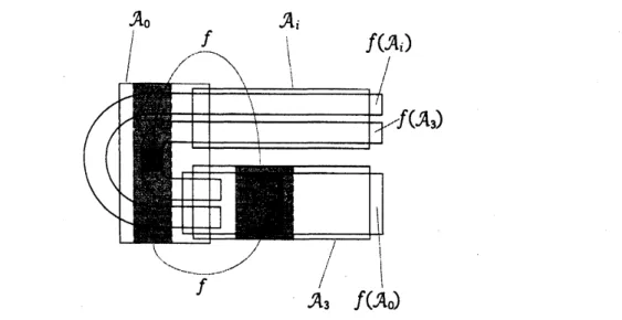
field $(\{C_{p}^{\cap}\}_{p\in A}, ||\cdot||_{\cap})$

by using $\{C_{p}^{A_{i}}\}_{p\in A}.\cdot$ See Figure 1 below, where we described how the boxes

are

sitting in

$\mathbb{C}^{2}$, how

they

are

overlapped and how they are mapped by $f$. The shaded regions

are

the

holes of$A_{0}$and $A_{3}$ andtheirimages. Note that thetwo disjoint Poincar\’eboxes _{$A_{i}(i=1,2)$}

are

figured out in the

same

place in Figure 1.

With ahelp ofrigorous numerics technique described inthe previous section we

are

able

to get the

Proposition 7.1. There are 10 programs written in $C++which$ rigorously verzfy the

fol-lowing assertions using interval arithmetic: (i) $J_{j}\subset A$

,

(ii) The following transitions: $A_{0}arrow A_{3},$ $A_{1}arrow A_{0},$ $A_{1}arrow A_{1f}A_{1}arrow A_{2f}A_{2}arrow A_{0}$,

$A_{2}arrow A_{1},$ $A_{2}arrow A_{2},$ $A_{3}arrow A_{0},$ $A_{3}arrow A_{1}$ and $A_{3}arrow A_{2}$ by $f$ satisfy the $(BCC)$ and the $(OCC)_{\rangle}$

(iii) There exists a bidisk$\mathcal{V}\supset\bigcap_{|n|\leq 2}f^{n}(A_{0}\cap A_{3})$ so that $f$ : $\mathcal{V}arrow \mathcal{V}$

satisfies

the $(BCC)$

of

degree one.

Combining this propositionwith Corollary4.8 and the Gluing Lemma,

one can

conclude that the cubic H\’enon map $f_{a,b}$ is hyperbolic

on

its Julia set.

To conclude the proof, we show that $f_{a,b}$ is not topologically conjugate to a small

per-turbation of any hyperbolic polynomial in

one

variable. Assume that $f=f_{a,b}$ is conjugate

to

a

small perturbation $g=f_{q,b}$ of

some

expanding polynomial $q$. The degree of $q$ then

should be three,

_so

_it has two critical points. If both of their orbits diverge to infinity, then $J_{\mathit{9}}$ is totally disconnected. However, $J_{f}$ contains solenoids of period two, so this is

not the

case.

If both of their orbits

are

bounded, then $J_{g}$ is

connected.

However, $J_{f}$ is not

connected (note that the transitions $A_{i}arrow A_{0}$ for $i=1,2$ look like a horseshoe),

so

this is not the case either. Thus, the only possibility is that

one

orbit

converges

to

an

attractive cycle and the other diverges to infinity. Note that, by compareing the number of periodic points, one sees that $q$has aunique attractive cycleofperiod two, which attracts a critical

orbit. For two among thethree fixedpoints of$f$, the connectedcomponent of$J_{f}$ containing

the fixed point consists of the point itself. For two

among

the three fixed points of $g$, the

connected component of $J_{g}$ containing the fixed point is homeomorphic to the projective

limit $\lim_{arrow}(p, J_{p})$, where $p(x)=x^{2}-1$

.

It follows that $f$

can

not be topologically conjugate to $g$

on

their Julia sets. This finishes the proofof Main Theorem. Q.E.D.

For

more

details of the proof, consult [I].

REFERENCES

[BS1] E. Bedford, J. Smillie, Polynomial diffeomorphisms _of$C^{2}$: Currents, equilibrium measure and

hyperbolicity. Invent. Math. 103, no. 1, 69-99 (1991).

[BS7] B. Bedford, J. Smillie, Polynomial diffeomorphisms _of$C^{2}$. VII: Hyperbolicity and extemal rays.

Ann. Sci. \’EcoleNorm. Sup. 32,no. 4, 455-497 (1999).

[D] A.Douady, Descriptions_ofcompactsetsinC.Topological Methods in Modern Mathematics(Stony

Brook, NY, 1991),429-465, Publishor Perish, Houston, TX, (1993).

[FS] J. E. Fornaess, N. Sibony, Complex H\’enon mappings in $C^{2}$ and Fatou-Bieberbach domains. Duke

Math. J.65, no. 2, 345-380 (1992).

[FM] S.Friedland, J. Milnor, Dynamicalproperties_ofplane polynomial automorphisms. Ergodic Theory Dynam. Systems 9, no. 1, 67-99 (1989).

[HO1] J. H. Hubbard, R. W. Oberste-Vorth, H\’enon mappings in the complex domain. I.. The global topology

_of

dynamical space. Inst. Hautes\’Etudes Sci. Publ. Math. 79, 5-46 (1994).

[HO2] J. H. Hubbard, R. W. Oberste-Vorth, H\’enon mappings in the complex domain. II.. Projective and inductive limits

_of

polynomials. Real and Complex Dynamical Systems (Hillerod, 1993), 89-132,

NATO Adv. Sci. Inst. Ser. C464, KluwerAcad. Publ., Dordrecht (1995).

[I] Y. Ishii, Hyperbolic polynomial diffeomorphisms _of$\mathbb{C}^{2}$. Preprint (2005).