Interaction between self-sustained flow oscillations and acoustic waves in a hole-tone system with an attached tailpipe (Mathematical Aspects and Applications of Nonlinear Wave Phenomena)

Interaction between self-sustained

flow

oscillations

and

acoustic

waves

in

a

hole-tone

system with

an

attached

tailpipe

Mikael A. Langthjem\dagger and Masami Nakano\ddagger

\dagger

Graduate School

of

Science

and Technology, Yamagata

University,

Jonan 4-chome, Yonezawa-shi,

992-8510

Japan

\ddagger Institute _{of Fluid Science, Tohoku University,}

2-1-1

Katahira, Aoba-ku, Sendai-shi,

980-8577

Japan

Abstract

This paper is concerned with a mathematical model of asimple axisymmetric silencer-like

model, consisting ofa hole-tone feedback system equippedwithbyatailpipe. The unstable

shear layer is modeled via a discrete vortex method, based on axisymmetric vortex rings.

The aeroacoustic model is based on the Powell-Howe theory of vortex sound. Boundary

integrals _{are discretized viathe boundary element method; but the tailpipe is represented}

by the exact _{(one-dimensional) solution. It is demonstrated though numerical examples that}

thisnumerical$mo$delcandisplay$10$ck-inof theself-sustainedflow oscillations to the resonant

acousticoscillations.

1

_Introduction

Expansion chambersare oftenused in connection withsilencers in engineexhaust systems, with

the aim of attenuating the energy flow. But the gas flow through the chamber may generate

self-sustained oscillations, thus becoming a sound generator rather than a sound attenuator.

Similar geometries _{and thus similar} problems may be found in, for example, solid propellant

rocket motors, valves, and heat exchangers.

The present work is related to a simple axisymmetric silencer model consisting of an

ex-pansion chamber followed by a tailpipe. The aim is to contribute to the understanding of the

interaction between oscillations of the flow field and the acoustic field.

By_{oscillations of the flow field we mean the self-sustained oscillations of thejet shear layer.}

The shear layer is unstable and rolls up into alarge, coherent vortex (a ‘smoke-ring’) which is

convected downstream withthe flow. It cannot pass through the hole inthe downstream plate

but hits the plate, where it creates a pressure disturbance. The disturbance is ‘thrown’ back

(withthespeedof sound) to theupstream plate,where it disturbs the shearlayer. This initiates

the roll-up ofa new coherent vortex. In this way an acoustic feedback loop is formed, making

up onetype offlow-acoustic interaction.

These so-called hole-tone feedback oscillations may interact with the acoustic axial and

radial eigen-oscillations of the cavity and the tailpipe. It is these interactions that we seek to

understand. In the present paper we study thesimplified configuration shown in Fig. 1. This is

Figure 1: The hole-tone feedback system witha tailpipe. The

arrow

indicates the direction of the flow.

The unstable shear layer is modeled viaadiscrete vortex approach, based on axisymmetric

vortex rings. The aeroacoustic model is based

on

thePowell-Howetheory ofvortex sound [4, 5].

Theboundary integrals that appear

are

discretized via the boundary element method.

The present paper concentrates on the aeroacoustic analysis. $A$ description of the flow

analysis (discrete vortex method) has been given in earher papers [8, 9]. The geometry of the

problemfacilitates the use of cyhndrical polar coordinates $(r, \theta, z)$, withthe fluid flowing inthe

positive $z$-direction. Although it is possible that non-axisymmetric modes may be excited, we

will, at this stage, consider onlythe axisymmetric modes $(r, z)$

.

The paper is organized

as

follows. The aeroacoustic model and its solution is described

in Section 2. Section 3 considers details related to the boundary element discretization. The

boundary element grid, and the representation of the tailpipe, isdiscussed in Section 4. Details

regarding thesolutionofthe tailpipe problem andthe acoustic feedback modelare discussedin

Section 5. Numerical examples

are

given and discussed in Section 6. Finally, conclusions

are

given in Section 7.

2

Vortex sound

Modelingofthe flow-induced soundis based on Howe’s equation for vortex sound at low Mach

numbers [4, 5]. Let $u$ denote the flow velocity, $\omega=\nabla\cross u$ the vorticity, $c0$ the speed ofsound,

and$\rho_{0}$ the the

mean

fluiddensity. The soundpressure$p(x, t)$at the position$x=(r, z)$ and time

$t$is relatedtothe vortex force (Lamb vector)$\mathfrak{L}(x, t)=\omega(x,t)\cross u(x, t)$ viathe non-homogeneous

wave equation

$( \frac{1}{c_{0}^{2}}\frac{\partial^{2}}{\partial t^{2}}-\nabla^{2})p=\rho 0\nabla\cdot \mathfrak{L}$, (1)

with boundary conditions $\partial p/\partial n=\nabla p\cdot n=0$ on the solid surfaces ($n=$ normal vector), and

$parrow 0$ for $|x|arrow\infty.$

To solve (1) and (2) in an axisymmetric setting, use is made of the free-space time-domain

axisymmetric Green’s function $G(t, \tau;r, z;r_{*}, z_{*})$, which isasolution to

$- \frac{1}{A}\frac{\partial^{2}G}{\partial t^{2}}+\frac{\partial^{2}G}{\partialr^{2}}+\frac{1}{r}\frac{\partial G}{\partial r}+\frac{\partial^{2}G}{\partial z^{2}}=-\frac{\delta(r-r_{*})}{r}\delta(z-z_{*})\delta(t-\tau)$, (2)

where $\delta$ is Dirac’s delta function. It can be shown that the solutionis given by

$G(t, \tau;r, z;r_{*}, z_{*})=\frac{c_{0}}{\pi}\frac{H(f_{n}^{+})H(f_{\overline{n}})}{\sqrt{f_{d}^{+}f_{d}^{-}}}$ , (3)

where

and

$f_{d}^{+}=(r+r_{*})^{2}+(z-z_{*})^{2}-c_{0}^{2}(t-\tau)^{2},$ $f_{d}^{-}=c_{0}^{2}(t-\tau)^{2}-(z-z_{*})^{2}-(r-r_{*})^{2}$

.

(5)

Here $H(f)$ _{is the Heaviside unit function which takes the value 1 when $f>0$ and the value} $0$

when $f<0.$

By making use of the Green’s function, the pressure$p(x, t)$ at any point _{$x=(r, z)$} can _be

determined

as

$p(t, r, z)=- \rho_{0}l\{\int_{z_{*}}l_{*}\nabla_{y}G\cdot \mathfrak{L}r_{*}dr_{*}dz_{*}+\int_{z_{*1}}^{z_{*2}}(p_{*}\frac{\partial G}{\partial r_{*}}-G\frac{\partial p_{*}}{\partial r_{*}})2\pi r_{*}dz_{*}$ (6)

$+ \int_{r_{*1}}^{r_{*2}}(p_{*}\frac{\partial G}{\partial z_{*}}-G\frac{\partialp_{*}}{\partial z_{*}})2\pi r_{*}dr_{*}\}d\tau,$

where, in the first term, $\nabla_{y}=(\partial/\partial r_{*}, \partial/\partial z_{*})$. This (first) term represents the ‘source’

contri-bution $p_{s}$ from the vortex rings. The vorticity related to asingle ring is given by

$\omega_{j}=\Gamma_{j}\delta(r_{*}-r_{j})\delta(z_{*}-z_{j})i_{\theta}$, (7)

where $i_{\theta}$ is a unit vector in the azimuthal direction of the

cylindrical polar coordinate system

$(r, \theta, z)$

.

Then, by making use of _{$(3, 4)$}, the first term in (6) takes the form

$p_{s}= \frac{c_{0}}{\pi}\rho_{0}\sum_{j}\{sgn(r, r_{j})\frac{\partial t}{\partial r,t-}\int_{d_{j}^{+}/c0}^{-d_{j}^{-}/c_{0}}\frac{\Gamma_{j}(\tau)v_{zj}(\tau)r_{j}}{\sqrt{f_{d}^{+}f_{d}^{-}}}d\tau-sgn(z, z_{j})\frac{\partial}{\partial z,t-}\int_{d_{j}^{+}/c0}^{t-d_{j}^{-}/c0}\frac{\Gamma_{j}(\tau)v_{rj}(\tau)r_{j}}{\sqrt{f_{d}^{+}f_{d}^{-}}}d\tau\}$ , (8)

where the subscript $s$’ stands for ‘source term’. The summation over $j$ refers to summation

over all free vortex rings. Note that differentiation with respect to the source variables $r_{j}$ and

$z_{j}$ have been converted into differentiation with respect to _$r$ and _$z$. Here care should be taken

with the signs related to $r_{j}$ and $r$ and to$z_{j}$ and $z$; see (4) and (5). This is taken careof by the

functions sgn$(r, r_{j})$ and sgn$(z, z_{j})$.

The main contributions to the $\tau$-integrations will be at the end point singularities. Hence

the functions $f_{d}^{+}$ and$f_{d}^{-}$ can be approximated as

$f_{d}^{+}\approx 2c_{0}d_{j}^{+}\{\tau-(t-d_{j}^{+}/c_{0})\}, f_{d}^{-}\approx 2c_{0}d_{j}^{-}\{(t-d_{j}^{-}/c_{0})-\tau\}$, (9)

where

$d_{j}^{+}=\{(r+r_{j})^{2}+(z-z_{j})^{2}\}^{\frac{1}{2}}, d_{j}^{-}=\{(r-r_{j})^{2}+(z-z_{j})^{2}\}^{\frac{1}{2}}$

.

₍₁₀₎

Let $a=t-d_{j}^{+}/c_{0}$ and $b=t-d_{j}^{-}/c_{0}$

.

The integralsover $\tau$ in (8) then take the form

$I_{\mathcal{T}}(t)= \int_{a}^{b}\frac{F(\tau)}{\sqrt{(\tau-a)(b-\tau)}}$, (11)

which is a standard Gauss-Chebyshev integral. The corresponding quadrature formula isgiven

by

where $R_{I}$ is the reminder. Using just

one

point, i.e. taking $I=1$, corresponds to assuming

that the vortex strengths $\Gamma_{j}(\tau)$ and the corresponding velocities $v_{rj}(\tau, r_{j}, z_{j}),$ $v_{zj}(\tau, r_{j}, z_{j})$

are

constant within the limits of integrationover $\tau$, andequal totheir values at the meanretarded

time $\overline{t}=t-(d_{j}^{+}+d_{j}^{-}))/2c_{0}$

.

Applying this approximation,

an

evaluation of (8) gives

$p_{s}=- \frac{\rho_{0}}{4}\sum_{j}\frac{r_{j}}{\sqrt{d_{j}^{+}d_{j}^{-}}}[\Gamma_{j}v_{zj}(tJ\{\frac{r+r_{j}}{(d_{j}^{+})^{2}}-\frac{r-r_{j}}{(d_{j}^{-})^{2}}\}+\Gamma_{j}v_{rj}(tJ(z-z_{j})\{\frac{1}{(d_{j}^{+})^{2}}+\frac{1}{(d_{j}^{-})^{2}}\}$ (13)

$+ \frac{1}{c_{0}}\frac{\partial}{\partial\overline{t}}(\Gamma_{j}v_{zj}(\overline{t}))\{\frac{r+r_{j}}{d_{j}^{+}}-\frac{r-r_{j}}{d_{j}^{-}}\}+\frac{1}{c_{0}}\frac{\partial}{\partial\overline{t}}(\Gamma_{j}v_{rj}(t\gamma)(z-z_{j})\{\frac{1}{d_{j}^{+}}+\frac{1}{d_{j}^{-}}\}].$

The second and third terms of (6) make up the scattering contribution $p_{sc}$, due to the solid

surfaces. We use the subscript $sc$’ to refer to ‘scattered’, and the subscript asterisk in $p_{*}$ to

refer to the surface pressure. The second term is for the horizontal sections (integration along

the $z$ axis) while the third term is for the vertical surfaces (integration along the $r$ axis). By

making use of the same kind of approximations

as

applied to the vortex source term$p_{s}$ these

terms canbe evaluatedas

$p_{S\mathcal{C}}= \frac{\pi}{2}\delta_{hc}\int_{z_{*1}}^{z_{*}}\frac{2r}{\sqrt{d_{*}^{+}d_{*}^{-}}}*[p_{*}(tJ\{\frac{r+r}{(d_{*}^{+})^{2}}*-\frac{r-r_{*}}{(d_{*}^{-})^{2}}\}+\frac{1}{c_{0}}\frac{\partial}{\partial\overline{t}}(p_{*}(t\gamma)\{\frac{r+r}{d_{*}^{+}}*-\frac{r-r_{*}}{d_{*}^{-}}\}]dz_{*}$ (14) $- \frac{\pi}{2}\delta_{vc}l_{1}^{r_{r2}}\frac{r_{*}(z-z_{*})}{\sqrt{d_{*}^{+}d_{*}^{-}}}[p_{*}(t]\{\frac{1}{(d_{*}^{+})^{2}}+\frac{1}{(d_{*}^{-})^{2}}\}+\frac{1}{c_{0}}\frac{\partial}{\partial\overline{t}}(p_{*}(t\gamma)\{\frac{1}{d_{*}^{+}}+\frac{1}{d_{*}^{-}}\}]dr_{*}$

$+ \pi\delta_{ho}\int_{z_{*1}}^{z.2}\frac{r}{\sqrt{d_{*}^{+}d_{*}^{-}}}*\frac{\partial p_{*}(tJ}{\partial r_{*}}dz_{*}+\pi\delta_{vo}lt_{1}^{2}\frac{r}{\sqrt{d_{*}^{+}d_{*}^{-}}}*\frac{\partial p_{*}(t\ovalbox{\tt\small REJECT}}{\partial z_{*}}dr_{*}.$

Here $\delta_{hc}$ is 1 on horizontal closed (i.e. physical) surfaces, and $0$ otherwise; $\delta_{vc}$ is 1 on vertical

closed surfaces, and $0$ otherwise; $\delta_{ho}$ is 1 on horizontal open (i.e. virtual, or control) surfaces,

and $0$ otherwise; and$\delta_{vo}$ is 1 on vertical open surfaces, and $0$ otherwise.

The total pressure at an observation point $(r, z)$ is now given by

$\sigma p(\overline{t}, r, z)=p_{s}(\overline{t}, r, z)+p_{sc}(\overline{t}, r, z)$

.

(15)

Here $\sigma$ is equal to 1 when the observation point is in the acoustic medium and away from the

solid boundaries, and equalto $\frac{1}{2}$ when the observation point is located on a sohd boundary.

3

Boundary

element

discretization

Next we employ the boundary element methodology of dividing the surface into $V$ elements,

assuming that the pressure is constant within each element. The time dependence of the

pres-sure is, within cosecutive time steps, interpolated via a cubic polynomial. Thus, the pressure

anywhere on the boundary$p_{*}(tJ$ can, at time step $W$, be expressed

as

$p_{*}( \overline{t}, r_{*}, z_{*})=\sum_{v=1}^{V}\sum_{w=1}^{W}f_{v}(r_{*}, z_{*})g_{w}(t\gamma P_{vw},$ (16)

where

and$g_{w}(t\gamma=g(t-w\Delta t)$, with

$g(t)=\{\begin{array}{ll}1+\frac{11}{6}\frac{t}{\Delta t}+(\frac{t}{\Delta t})^{2}+\frac{1}{6}(\frac{t}{\Delta t})^{3} for -At\leq t<0,1+\frac{1}{2}\frac{t}{\Delta t}-(\frac{t}{\Delta t})^{2}-\frac{1}{2}(\frac{t}{\Delta t})^{3} for 0\leq t<\Delta t,1-\frac{1}{2}\frac{t}{\Delta t}-(\frac{t}{\Delta t})^{2}+\frac{1}{2}(\frac{t}{\Delta t}I^{ 3} for \Delta t\leq t<2\Delta t,1-\frac{11}{6}\frac{t}{\triangle t}+(\frac{t}{\Delta t})^{2}-\frac{1}{6}(\frac{t}{\Delta t})^{3} for 2\Delta t\leq t<3\Delta t,0 otherwise. \end{array}$

(18)

In the usual collocation type BEM (14) is evaluated at each of the $V$ spatial control points

in turn, to give $V$ equations for the $V$ unknown element pressures (at each time step). Here

weemploy the Galerkinmethod, where the ‘strong form’ oftheseequations areexchanged with

a ‘weak form’. To this end, (14) is multiplied by the spatial shape function $f_{u}$, followed by

integration around theclosed surface (see also Section4). Letting$u$ runfrom 1 to $V$, we obtain

a$V\cross V$ equation system on the form

$A_{0}p_{W}=-\sum_{w=1}^{N_{save}}A_{w}p_{W-w}+f_{W}$, (19)

which issolved at eachtimestep.

4

Boundary

element

grid and tailpipe representation

The closed surface, _{which is assumed when applying Green’s second identity [7] to convert}

volume integrals into surfaceintegrals in(6), canbe specified in avariety of ways. The standard,

and most simple, way would be to represent the solid surfaces by boundary elements, making

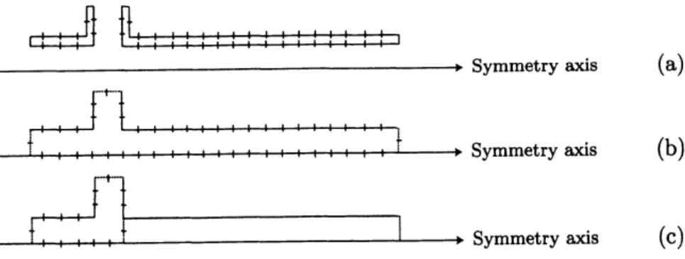
two separated closed surfaces in the present case, as shown in Fig. 2 (a). This approach

has the benefit that the terms proportional to $\partial p_{*}/\partial r_{*}$ and $\partial p_{*}/\partial z_{*}$ in (14) drop out. But

it makes internal

resonances

possible. This will in turn imply a numerical instability that

is difficult to cure. $A$ number of methods to circumvent this problem are available,

such as

the methods known as CHIEF (Combined Helmholtz Integral Equation Formulation) [10] and

CONDOR (CompositeOutward Normal Derivative Overlap Relation) [1]. Both of thesemethods

were developed originally for frequency-domain formulations but can be modified to be used in

the time domain. Such modificationshave been considered for the CONDORmethod by $[[3]]$ and

[2] and also, very recently, for the CHIEF method by [6].

We have tried to use the latter approach in connection with a grid layout as that shown

in Fig. 2 (a) but did not obtain sufficient stabilization. Accordingly, the grid was modified to

one as shown in Fig. 2 (b). Here the acoustic medium within the whole hole-tone$/pipe$ system

is surrounded by elements; and the resonances that can occur within the closed surface are

the physical

resonances

that we are interested in. Yet is was found to be difficult to stabilize

thevibrations without damping out the

resonance

peaks too much. On another note, it

can

be

arguedthat, since the acoustic

waves

inthetailpipe principally

are

one-dimensional, aboundary

element representation of this long, slender surface is ‘wasteful’ from a computational point of

view. Theseconsiderations, togetherwiththementionedstability problems, suggestanapproach

as that shown in Fig. 2 (c).

Here only the hole-tone-system part is represented by boundary elements. The pipe is

represented by the exact one-dimensional wave solution, considered as a ‘super element’, and

di

Symmetryaxis $($a$)$

(b)

(c)

Figure 2: Possible boundary element grids. Dotted lines indicate open (pressure rehef)

bound-aries.

5

Pressure

in the

tailpipe

and

acoustic

feedback

Let $z=z_{1}$ correspond to the upstream pipe entrance and $z=z_{2}$ to the downstream pipe exit.

Inthe following wewill

use

the local coordinate $\tilde{z}=z-z_{1}$

.

Also, let $\ell=z_{2}-z_{1}.$

We will

assume

that the ‘driving’ disturbance at $\tilde{z}=0$

can

be described in terms of its

velocity potential there, $\phi_{0}$ say. Next we will evaluate the velocity potential $\phi$ inthe pipe. Use

of the velocitypotential is convenient because once it $(\phi)$ is known the acoustic pressure$p$ and

particle velocitycan be determined

as

$p= \rho 0\frac{\partial\phi}{\partial t}, u=-\frac{\partial\phi}{\partial z}$. (20)

The numerical evaluation of $\phi_{0}$ is based on the pressure gradient at the $BEM$-pipe interface,

$(\partial p/\partial z)_{z=z}1^{\cdot}$

In the frequency domain, the Green’s function corresponding to a disturbance at $\tilde{z}=0$, of

unit amplitude and frequency $\omega$, takes the form

$\tilde{G}_{\phi}=\frac{\sin k(\ell-\tilde{z})}{\sin k\ell}$ (21)

where $k=\omega/c_{0}$

.

The time-domain version of this equationtakes the form

$G_{\phi}= \sum_{n=0}^{\infty}[\delta(t-\frac{\tilde{z}+2n\ell}{c_{0}})-\delta(t+\frac{\tilde{z}-2(n+1)\ell}{c_{0}})]$, (22)

where $\delta$ is the (Dirac) delta function. Based on this Green’s functionwe get

$\phi(t,\tilde{z})=\sum_{n=0}^{\infty}[\phi_{0}(t-\frac{\tilde{z}+2n\ell}{c_{0}})-\phi_{0}(t+\frac{\tilde{z}-2(n+1)\ell}{c_{0}})]$

.

(23)

In order evaluate the acoustic particle velocity radiated from the pipe it will, for simplicity

andas$a$ first approximation’, be assumedthat the one-dimensionalvelocity field inside the pipe

is radiated out inthe

same

one-dimensional way. That is, if$z_{1+}$ is apoint a little downstream

from the pipe entrance at $z_{1}$ the acoustic particle velocity at value of$z<z_{1}$ is evaluated

as

$u(z, t)=u(z_{1+}, t-(z_{1+}-z)/c_{0})$ (24)

The acoustic velocity field is superimposed onto the ‘hydrodynamic’ velocity field of the free

vortexrings in the open domain between nozzle exit and end plate. That is, (24) is evaluated

6

Numerical

examples

In the numerical examples to follow the diameters ofnozzle, endplate hole, andtailpipe areall

$d_{0}=50$mm. The gap length between_{nozzle exit and the endplateis also50mm. The diameter}

ofthe end plateis3$d_{0}=150$mm. Themeanjet _{speed$u_{0}=10m/s$}. _{The (reference) length ofthe}

tailpipe attached onto the end plate is$\ell=21.25d_{0}=1063$mm. The _{corresponding (reference)}

pipe

resonance

frequencies are $f_{n}=160n,$ _$n=1,2,$$\cdots$, where even values of_$n$ correspond to

multiples ofa full wavelength.

Thetime step is chosen as $\Delta t=1/(10f_{\max})$ where the maximum frequency ofinterest $f_{\max}$

is set to 1100Hz. Thenumber of boundary elements on a certain ‘stretch’ oflength $l_{i}$ (between

two corners) is set to $N_{e}= \max[2, \{nint(4l_{i}/(c_{0}\triangle t))\}].$

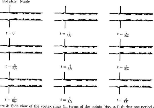
Figure 3 shows the appearance and location of free vortex rings in the vicinity of the end

plateduring oneperiod ofoscillation. Thefundamental hole-tone frequency $f_{0}=158$Hz, which

is about 40Hz lower than for the

case

without

a

tailpipe [8, 9]. The change in $f_{0}$ is due to the

different flow field that the tailpipe causes.

Endplate Nozzle

$t=0$ $t= \frac{1}{8f_{0}}$ $t= \frac{2}{8f_{0}}$

$\underline{--\frac{1}{--}} ---\underline{\frac{1}{*\vee}}$

$t= \frac{3}{8f_{0}}$ $t= \frac{4}{8f_{0}}$ $t= \frac{5}{8f_{0}}$

$-|$

–

$t= \frac{6}{8fo} t=\frac{7}{8fo} t=\frac{8}{8f_{0}}$

Figure 3: Side view of the vortex rings $(in$ terms _{$of the$} points $(\pm r_{j}, z_{j})$) during one period of

oscillation.

Figure 4 shows anumber of time series plots for the pressurevariationonthe axis of

symme-try, in the middle ofthe tailpipe. It is noted that this position corresponds to a nodal point for

the even modes $n=2,4,$$\cdots$ . Thus in the corresponding sound pressure spectra (Fig. 5), only

thepeaks at $f_{2n-1},$ $n=1,2,$$\cdots$, correspondto pipe resonances; the peaksat _{$f_{2n}$} correspondto

thehole-tone oscillations.

In bothofthese twofigures (4 and5) the sub-plotsonthe left-handsideare for caseswithout

acoustic feedback; those on the right-hand sideare for cases with acoustic feedback.

In the time series plot of Fig. 4 (a) the hole-tonefrequency $(f_{0}=158 Hz)$ _{is close to the first}

Withoutacoustic feedback Pressure$p/p_{0}$ 3 2 1 $0$ $-1$ $-2$ 3 $0$ $0.\infty$ Ot 015 02 $OX$ ₀₃ $(a)$ 15 1 $05$ $0$ $\langle)5$ $-1$ -t 5 $0$ $0\propto$ 01 015 $0l$ $0X$ 0.$3$ $(c)$ 15 1 $05$ $0$ $05$ $\sim t$ $-15$ $0$ 15 1 0.5 $0$ $05$ $-1$ $-15$ $0$

With acoustic feedback

0._$3(f)$

$0.3(h)$

$os$ 05

$4!5$ 15

$-/ \sim 1$

$0$ OOS OI 015 02 $OX$ 03 _$(i)$ $0$ $0oe$ Ot 015 02 025 03 $(j)$

Time $[s]$ Time $[s]$

Figure 4: Sound pressure time series. [Reference pressure$p_{0}= \frac{1}{2}\rho_{0}u_{0}^{2}.$] The observationpoint

is on the jet axis, in the middle of the pipe. The sub-plots on the left-hand side are for

cases

without acoustic feedback; thoseonthe right-hand sidearefor caseswithacoustic feedback. $(a,$

b$)$ Pipe length $\ell=21.25d_{0}.$ $(c, d)\ell=22.25d_{0}.$ $(e, f)\ell=23.25d_{0}.$ $(g, h)\ell=20.25d_{0}.$ $(i, j)$

$\ell=19.25d_{0}.$

to it. For this reason a slow beat phenomenon, withaperiod of0.5$s$, is developed.

When acoustic feedback is included (Fig. 4 $(b)$) the hole-tone oscillations lock-in to the

pipe oscillations, and a clear resonance is developed. The pressure amplitude grows to large

values in a almost linear fashion. As a reference, it is noted that the amphtude of a simple,

undamped, forced one degree-of-heedom oscillator grows linearly; so the behavior in Fig. 4 (b)

appears plausible. Comparing the spectra of Fig. 5 (a) and (b) it is seen that peaks of $f_{2n-1}$

$(n=1,2, \cdots)$ areraised significantly bythe feedback.

Theplotsin Figs. 4 and 5, parts (c) and(d), are forapipeof length$\ell=22.25d_{0}$

.

This gives

the resonance frequencies $f_{n}=151n,$ $n=1,2,$$\cdots$ . The larger difference between $f_{0}$ and $f_{1}$

imphes faster beats, as seen from Fig. 4 (c). Inclusion of acoustic feedbackgives, instead ofthe

beats, again an almost linear pressure amplitude growth (Fig. 4 $(d)$) -which however ‘flattens

off’ at larger times.

Without acousticfeedback

SPL $[dB]$

With acoustic feedback

SPL $[dB]$

$0 200 400 600$

800 _(i) $0$ 200 $4\infty$ 600 800

(j)

Time $[s]$ Time $[s]$

Figure 5: Sound pressure spectra of the time series shown in Fig. 4. [Sound pressure level

(SPL) in $dB$; reference pressure _{$p_{ref}=2\cross 10^{-5}N/m^{2}.$] Again, the sub-plots onthe left-hand}

side are for cases without acoustic feedback; those on the right-hand side are for cases with

acoustic feedback. $(a, b)$ Pipe length $\ell=21.25d_{0}.$ $(c, d)\ell=22.25d_{0}.$ $(e, f)\ell=23.25d_{0}.$ $(g, h)$

at 2$f_{0}\approx 320$Hz moves to 2$f_{0}\approx 300$Hz$\approx 2f_{1}$ when acoustic feedback is included. That is to

say, the hole-tone frequency $f_{0}$ undergoes

a

$10$ck-in to the pipe

resonance

frequency $f_{1}.$

Figures 4 and 5, parts (e) and (f), show that lock-in of$f_{0}$ to $f_{1}$ happens also when feedback

isincluded for apipe abit longer, oflength$\ell=23.25d_{0}$, with

resonance

frequencies $f_{n}=146n.$

Here the pressure amplitude grows linearly only for small values of time $t$; at larger times it

takes an almost-constant value.

Shorter pipes that have

resonance

frequencies $f_{n}>f_{0}$ have been considered

as

well (Figs.

4 and 5, parts $(g)-(j))$

.

But here the acoustic feedback does not easily imply a lock-in of the

hole-tone frequency to that of the pipe

resonance.

More computational studies are needed in

order to identify andunderstand regions (inthe parameter space) with lock-inand non-lock-in.

It must be pointedout, lastly, that the magnitudeofthefeedback velocity field is important,

and that

one

can

hardly expect the present simple approach to give the correct magnitude. In

thenumerical examples presentedhere, an‘amplificationfactor’ (multiplier) wa.$s$used to enlarge

the numerical value of thevelocity. For the pipe lengths$\ell=19.25d_{0}$, 20.25$d_{0}$, and 21.25$d_{0}$, the

amplification factor was 25; for $\ell=22.25d_{0}$ and 23.25$d_{0}$, it was 50.

7

Conclusions

1. Use of a discrete vortex method in combination with the theory of vortex sound and

the boundary element method has proved to be an efficient and computationally

sim-ple approach for simulation of flow-acoustic interaction problems, like the hole-tone/pipe

resonance problem considered here.

2. The employed time-domainboundaryelement methodcanbe made numericallystable;but

(physical, pipe)

resonances

within the closed boundary domain triggerinstabilityproblems.

Use of theanalytical solutionfortheacousticpipeoscillationscuresthe numericalstabihty

problem. It also reducesthe computational costs considerably.

3. Thenumerical model candisplay lock-in oftheself-sustained flow oscillations to the

reso-nant acoustic oscillations.

Acknowledgement: The work reported here was supported by a Collaborative Research

Project Grant (No. J13062) from the Institute ofFluid Science, Tohoku University.

References:

[1] A. J. Burton and G. F. Miller. Theapplicationof integral equation methods to thenumerical

solution ofsomeexterior boundary-valueproblems. Proc. Roy. Soc. Lond. (A),323:201-210,

1971.

[2] D. J. Chappell, P. J. Harris, D. Henwood, and R. Chakrabarti. A stable boundaryelement

method for modeling transient acoustic radiation. J. Acoust. Soc. Am., 120:74-80, 2006.

[3] A. A. Ergin, B. Shanker, and E. Michielssen. Analysis of transient wave scattering from

rigid bodies using aBurton-Miller approach. J. Acoust. Soc. Am., 106:2396-2404, 1999.

[4] M. S. Howe. Acoustics

_of

Fluid-Structure Interactions. Cambridge UniversityPress, 1998.

[6] H.-W. Jang and J.-G. Ih. Stabilization oftime domain acoustic boundary element method

for theexterior problem avoiding thenonuniqueness. J. Acoust. Soc. Am., 133:1237-1244,

2013.

[7] O. D. Kellogg. Foundations

_of

Potential Theory. Dover Publications, New York (1954

republication), 1929.

[8] M. A. Langthjemand M. Nakano. Numericalstudyof thehole-tone feedbackcyclebased on

an_{axisymmetric discrete vortex method and Curle’sequation. J. Sound Vibr., 288:133-176,}

2005.

[9] M. A. Langthjem and M. Nakano. A numerical simulation ofthe hole-tone feedbackcycle

basedon an axisymmetric formulation. Fluid Dyn. Res., 42:1-26, 2010.

[10] H. A. Schenck. Improved integral formulation for acoustic radiation problems. J. Acoust.