Optimality Conditions and Algorithms for Semi-Infinite Programs with an Infinite Number of Second-Order Cone Constraints (The evolution of optimization models and algorithms)

Optimality Conditions

and

Algorithms for

Semi-Infinite

Programs

with

an

Infinite

Number

of Second-Order

Cone

Constraints

奥野 貴之

(Takayuki Okuno)

林 俊介

(Shunsuke

Hayashi)

福島 雅夫

(Masao Fukushima)

京都大学大学院情報学研究科数理工学専攻

Department

of

Applied

Mathematics

and

Physics

Graduate School of

Informatics,

Kyoto

University

Abstract

The semi-infinite program (SIP) is normally represented with infinitely

many inequality constraints, and has been much studied so far. However,

there have beenveryfew studiesontheSIP involving second-ordercone(SOC)

constraints, eventhough it hasimportant applications suchas Chebychev-like

approximation and filter design.

In this paper, we focus on the SIP with a convex objective function and

infinitely many SOC constraints, called the SISOCP for short. We show

that, under a generalized Slater constraint qualification, an optimum of the

SISOCP satisfies the KKT conditions that can be represented only with a

finite

subset ofthe SOC constraints. Nextwe introduce theregularization and

the explicit exchange methods for solving the SISOCP. We first provide an

explicit exchange method withoutaregularizationtechnique, andshow that it

has globalconvergence under thestrictconvexity assumptiononthe objective

function. Then we propose an algorithm combining a regularization method

with the explicit exchange method. For the SISOCP, we establish global

convergence ofthehybrid algorithm without the strict convexityassumption.

1

Introduction

Inthis paper, we focus onthe following semi-infiniteprogramwithaninfinite number of second-order cone constraints:

Minimize $f(x)$

(1.1) subject to $A(t)^{T}x-b(t)\in \mathcal{K}$ for all $t\in T$

where $f$ : $\mathbb{R}^{n}arrow \mathbb{R}$ is

a

continuously

differentiable convex

function, $A:\mathbb{R}^{\ell}arrow \mathbb{R}^{n\cross m}$

and $b$ : $\mathbb{R}^{\ell}arrow \mathbb{R}^{m}$

are

continuous functions, $T\subseteq \mathbb{R}^{\ell}$ is

a

given compact set, and

$\mathcal{K}^{m_{i}}\subseteq \mathbb{R}^{m_{i}}(i=1,2, \ldots, s)$ is the second-order

cone

(SOC), that is, $\mathcal{K}$ $:=\mathcal{K}^{m_{1}}\cross$ $\mathcal{K}^{m}2\cross\cdots\cross \mathcal{K}^{m_{S}}$ with _{$m=m_{1}+m_{2}+\cdots+m_{s}$} and

$\mathcal{K}^{m:}:=\{\begin{array}{l}\{(x_{1},\tilde{x}^{T})^{T}\in \mathbb{R}\cross \mathbb{R}^{m_{i}-1}|x_{1}\geq\Vert\tilde{x}\Vert\} (m_{i}>1)\mathbb{R}_{+}=\{x\in \mathbb{R}|x\geq 0\} (m_{i}=1).\end{array}$

Throughout this

paper,

$\Vert\cdot\Vert$ denotes the Euclidean

norm

defined by $\Vert x\Vert$ $:=\sqrt{x^{T}x}$,

and $\tilde{v}$ denotes $(v_{2}, v_{3}, \cdots, v_{m_{i}-1})^{T}\in \mathbb{R}^{m_{i}-1}$ for $v=(v_{1}, v_{2}, \cdots, v_{m_{i}})^{T}\in \mathbb{R}^{m_{i}}$

.

For

simplicity,

we

will often write $(x_{1},\tilde{x})^{T}$ for $(x_{1}, x^{T})^{T}$.

We call the problem (1.1)

a

semi-infinite second-order

cone

problem (SISOCP).

One

of typical applications for SISOCP (1.1) is

a

Chebychev-like approximation withvector-valued functions. Let $Y\subseteq \mathbb{R}^{n}$ be

a

given compact set, and $\Phi$ : $Yarrow \mathbb{R}^{m}$ and $F$ : $\mathbb{R}^{\ell}\cross Yarrow \mathbb{R}^{m}$ begiven functions. Then, how

can we

determine

a

parameter $u\in \mathbb{R}^{\ell}$ such that _{$\Phi(y)\approx F(u, y)$} for all _{$y\in Y$}?

One

relevant approach is to solve

the following problem:

Minimizeu

$\max_{y\in Y}\Vert\Phi(y)-F(u, y)\Vert$ (1.2)

which

can

be rewritten

as

$Minimu,r$ize $r$

subject to $(_{\Phi(y)-F(u,y)}r)\in \mathcal{K}^{m+1}$ for all $y\in Y$

by introducing the auxiliary variable $r\in \mathbb{R}$. If $F$ is affine with respect to $u$, then

the above problem reduces to SISOCP (1.1) with $\mathcal{K}=\mathcal{K}^{m+1}$

.

When $m=1$ and $\mathcal{K}=\mathbb{R}_{+}$, SISOCP (1.1) is the classical semi-infinite program

(SIP) [3, 5, 8, 13, 15, 16], which has

a

wide application in engineering (e.g., the air pollution control, the robot trajectory planning, the stress of materials, etc.[8, 13]$)$

. So

far, many algorithms have been proposed for solving SIPs, such

as

the

discretization method [3], the local reduction based method [4, 11, 18] and the exchange method [5, 6, 16]. The discretization method solves the relaxed SIP with

$T$ replaced by

a

finite set $T^{k}\subseteq T$, and the sequence ofindex sets _$\{T^{k}\}$ is generated

so

that the

distancel

from $T^{k}$ to _$T$ converges to $0$

as

$k$ goes to infinity. While this

method is comprehensible and easy to implement, the computational cost tends to be huge sincethe cardinality of$T^{k}$ grows unboundedly. In the local reduction based

method, the infinite number ofconstraints in the SIPis rewritten

as

afinite number

of constraints with implicit functions. Although the SIP

can

be reformulated

as

a

finitely constrained optimization problem by this method, it is not possible in general to evaluate the implicit functions exactly in

a

direct

manner.

The exchange method solves

a

relaxed subproblem with $T$ replaced by

a

finite subset $T^{k}\subseteq T$

.

In

lFortwo sets$X\subseteq Y$, thedistance from$X$to$Y$is definedasdist_{$(X, Y)$ $:= \sup_{y\in Y}\inf_{x\in X}\Vert x-$}

this method, $T^{k}$ isupdated

so

that _{$T^{k+1}\subseteq T^{k}\cup\{t_{1}, t_{2}, \cdots, t_{r}\}$}with _{$\{t_{1}, t_{2}, \cdots, t_{r}\}\subseteq$} $T\backslash T^{k}$.

Studies

on

the second-order

cones

(SOCs) have been advanced significantly in the last decade. One of the most popular problems associated with SOCs is the linear second-order

cone

program (LSOCP). The primal-dual interior-point method [1, 12] is well known

as an

effective algorithmfor solving LSOCP, and

some

software

packages implementing them [17, 19] have been produced. The nonlinear second-order

cone

program (NLSOCP) [9, 10, 20] is more complicated and not studied

so

much

as

LSOCP. The second-order

cone

complementarity problem (SOCCP) is another important problem involving SOCs. The Karush-Kuhn-Tucker conditions for LSOCP and NLSOCP

are

particularly represented

as SOCCPs.

The smoothing method [2, 7] is

one

ofuseful algorithms for solving

SOCCP.

The main purpose of the paper is threefold. First, we provide the optimality conditionsfor SISOCP (1.1). The KKT conditions forSISOCP (1.1) could naturally be described by

means

of integration andBorel

measure

since $T$isinfinite. However,

we

show that, under

Slater’s

constraint qualification, the KKT conditions at the optimum

can

be represented by using

a

_finite

number of elements in $T$. Second,

we

propose

an

explicit exchange method for solving the SISOCP (1.1) and show its global convergence under the strict convexity of the objective function. Third, we propose

an

algorithm that

can

solve SISOCP (1.1) without the strict convexity. This

algorithmisahybridof the explicit exchangemethod andthe regularization method,

which is known to be effective in handling ill-posed problems. With the help of regularization,

a

global convergence of the algorithm

can

be established for

SISOCP

(1.1) without the strict convexity. As the notation usedinthis paper, $\mathcal{K}\ni x\perp y\in \mathcal{K}$

denotes the SOC complementarity condition, that is, $x^{T}y=0,$ $x\in \mathcal{K}$ and $y\in \mathcal{K}$

.

2

Karush-Kuhn-Tucker

Conditions

In this section, we show that the KKT conditions for

SISOCP

(1.1)

can

be rep-resented with finitely many second-order

cone

constraints. We first introduce the Slater constraint qualification (SCQ).

Definition 2.1 (SCQ). We say that the Slater Constraint Qualification (SCQ) holds

for

SISOCP

(1.1)

_if

there exists apoint $x_{0}\in \mathbb{R}^{n}$ such that$A(t)^{T}x_{0}-b(t)\in$ int$\mathcal{K}$

for

all $t\in T$.

Under the SCQ, the following theorem holds.

Theorem 2.2 (Theorem 2.12 [14]). Let $x^{*}\in \mathbb{R}^{n}$ be

an

optimum

of

SISOCP

(1.1)

and suppose that the $SCQ$ holds

for

SISOCP

(1.1). Then, there exist $p$ indices

$t_{1},$ $t_{2},$

$\ldots,$$t_{p}\in T$ and Lagmngian multipliers

$y^{1},$ $y^{2},$

$\ldots,$$y^{p}\in \mathbb{R}^{m}$ such that$p\leq n+1$, $\nabla f(x^{*})-\sum_{i=1}^{p}A(t_{i})y^{i}=0$,

3

Explicit

Exchange Method

In this section,

we

propose

an

explicit exchange method for solving

SISOCP

(1.1). Moreover,

we

show that the algorithm has

a

global convergenceproperty under mild assumptions. The algorithm proposed in this section requires solving second-order

cone

programs

(SOCP) with finitely

many

constraints

as

subproblems. Let

SOCP

$(T’)$ denote the relaxed problem

of

SISOCP

(1.1) with $T$ replaced by

a

finite subset

$T^{f}$ _{$:=\{t_{1}, t_{2}, \ldots, t_{p}\}\subseteq T$}. Then, the

SOCP

$(T^{f})$

can

be formulated

as

follows: Minimize $f(x)$

SOCP

$(T’)$

subject to $A(t_{j})^{T}x-b(t_{j})\in \mathcal{K}(j=1,2, \ldots,p)$

.

We suppose that the subproblem

SOCP

$(T’)$

can

be solved by any suitable existing

algorithm. Let $\overline{x}$be

an

optimal solution ofSOCP$(T’)$. Then,$\overline{x}$ satisfies the following

KKT conditions under

some

constraint qualification [1, 12]:

$\nabla f(\overline{x})-\sum_{t_{j}\in T’}A(t_{j})y_{t_{j}}=0$,

$\mathcal{K}\ni y_{t_{j}}\perp A(t_{j})^{T}\overline{x}-b(t_{j})\in \mathcal{K}(j=1,2, \ldots,p)$, (3.1)

where$y_{t_{j}}$ is

a

Lagrange multiplier vector corresponding to the constraint $A(t_{j})^{T}\overline{x}-$ $b(t_{j})\in \mathcal{K}$ for each $j$.

Now,

we

propose the following algorithm. Algorithm 1 (Explicit exchange method)

Step $0$

.

Chooseapositivesequence$\{\gamma_{k}\}\subseteq \mathbb{R}_{++}$ suchthat_{$\lim_{karrow\infty}\gamma_{k}=0$}

.

Choose

a

finite subset $E^{0}$

$:=\{t_{1}^{0}, \ldots, t_{p}^{0}\}\subseteq T$and solve

SOCP

$(E^{0})$ to obtain

an

optimal

solution $x^{0}$

. Set

$k:=0$

.

Step 1. Set $r:=0,$ $T_{0}:=E^{k}$ and $v^{0}:=x^{k}$. Do the following _$(a)-(c)$:

(a) Find

a

$t_{new}^{r}\in T$ such that

$A(t_{new}^{r})^{T}v^{r}-b(t_{new}^{r})\not\in-\gamma_{k}e+\mathcal{K}$

.

(3.2)

If such

a

$t_{new}^{r}$ does not exist, i.e.,

$A(t)^{T}v^{r}-b(t)\in-\gamma_{k}e+\mathcal{K}$ (3.3)

for any $t\in T$, then set $x^{k+1}$ _$:=v^{r},$ $E^{k+1}$ _{$:=T_{r}$}, and go to Step 2.

Otherwise, let

$\overline{T}_{r+1}:=T_{r}\cup\{t_{new}^{r}\}$,

and go to (b).

(b) Solve SOCP$(\overline{T}_{r+1})$ to obtain

an

optimum

$v_{r+1}$ and Lagrange multipliers

$y_{t}^{r+1}$, for $t\in\overline{T}_{r+1}$.

Step 2. If$\gamma_{k}$ is sufficiently small, terminate. Otherwise, set $k:=k+1$ and return to Step 1.

In Step l-(a), $e\in \mathbb{R}^{m}$ is defined

as

_{$e:=(e^{1}, e^{2}, \ldots, e^{s})^{T}$} and $e^{i}$ _{$:=(1,0, \ldots, 0)^{T}\in$}

$\mathcal{K}^{m_{i}}$. Toverify (3.3),

we

haveto solve acertain optimization problem

on

$T$ and check

the nonnegativity of the optimal value. For a detail, see [14]. Since this problem

is not necessarily convex, it is not easy to solve it. But, in this paper,

we

suppose that

we

can

obtain

a

global optimum of this problem every Step 1. In Step l-(b),

SOCP

$(\overline{T}_{r+1})$

can

be solved by applying

an

existing method such

as

the primal-dual

interiorpoint method, the regularized smoothing method, andso on [1, 2, 7, 10, 12]. In Step l-(c), SOCP$(T_{r+1})$ is obtained from SOCP$(\overline{T}_{r+1})$ by removing only the

constraints with

zero

Lagrange multipliers, then the optimal values of those two problems

are

equal. In addition, the feasible region of

SOCP

$(\overline{T}_{r+1})$ is contained in

that of

SOCP

$(T_{r})$. Therefore,

we have

$V_{P}(T_{0})\leq V_{P}(\overline{T}_{1})=V_{P}(T_{1})\leq\cdots\leq V_{P}(T_{r})\leq V_{P}(\overline{T}_{r+1})=V_{P}(T_{r+1})\leq\cdots\leq V_{P}(T)<+\infty$,

(3.4) where $V_{P}(T’)$ denotes the optimal value ofSOCP$(T’)$

.

Fortheproposedmethod to be welld-defined, Step 1 have to terminatein finitely

many iterations. To

ensure

this,

we

suppose the assumptions

as

follows:

Assumption A. i) Function $f$ is strictly

convex over

the feasible region ofSISOCP

(1.1). ii) In Step $1-(b)$ of Algorithm 1, SOCP$(\overline{T}_{r+1})$ is solvable for each $r.\ddot{\dot{m}}$)

A sequence generated $\{v^{r}\}$ in every Step 1 of Algorithm 1 is bounded. Under the Assumption $A$, the following theorem holds.

Theorem 3.1. [14, Theorem 4.1] Let that Assumption A hold. Then, the inner iterations in every Step 1

_of

Algorithm 1 terminate finitely.

Moreover,

we

have the following theorems for the globally convergent property. Theorem 3.2. [14, Theorem4.2] Let Assumption A hold. Let$x^{*}$ be the

optimum2

of

SISOCP (1.1), and $\{x^{k}\}$ be the sequence generated by Algorithm 1. Then, it

follows

that

$\lim_{karrow\infty}x^{k}=x^{*}$.

4

Regularized

Explicit

Exchange

Method

In the previous section,

we

proposedthe explicit exchange methodforSISOCP (1.1) and analyzed the convergence property. However, to

ensure

the global convergence, the strict convexity of the objective function

was

required (Assumption A). In this section,

we

propose

a

regularized explicit exchange method, and establish global convergence of the method without assuming the strict convexity.

Let $\epsilon$ be

a

positive number, and $T’:=\{t_{1}, t_{2}, \ldots, t_{p}\}$ be

a

finite subset of

$T$

.

The regularized explicit exchange method solves the following SOCP, denoted

SOCP

$(\epsilon, T’)$, in each

iteration.

Minimize $\frac{1}{2}\epsilon\Vert x\Vert^{2}+f(x)$

SOCP

$(\epsilon, T’)$ (4.1)

subject to $A(t_{j})^{T}x-b(t_{j})\in \mathcal{K}(j=1,2, \ldots,p)$

.

When the function $f$ is convex, $\frac{1}{2}\epsilon\Vert x\Vert^{2}+f(x)$ is strongly

convex.

Then, if

we

solve

SOCP

$(\epsilon_{k},\overline{T}_{r+1})$ with $\epsilon_{k}>0$instead of

SOCP

$(\overline{T}_{r+1})$ in Step l-(b) of Algorithm 1, it

is ensured by Theorem

3.1

that the inner iterations

terminate3

finitely. Moreover, by choosing positive sequences $\{\epsilon_{k}\}$ and $\{\gamma_{k}\}$ both converging to $0$, the generated

sequence is expected to converge to

a

solution of

SISOCP

(1.1). Now

we

propose the following algorithm for

SISOCP

(1.1).

Algorithm 2 (Regularized Explicit Exchange Method)

Step $0$

.

Choosepositivesequences $\{\gamma_{k}\}\subseteq \mathbb{R}_{++}$ and $\{\epsilon_{k}\}\subseteq \mathbb{R}_{++}$ suchthat$\lim_{karrow\infty}\gamma_{k}=$

$0,$ $\lim_{karrow\infty}\epsilon_{k}=0$ and $\gamma_{k}=O(\epsilon_{k})$. Choose

a

finite subset $E^{0}$ $:=\{t_{1}^{0}, \ldots, t_{l}^{0}\}\subseteq$ $T$.

Set

$k$ _$:=0$

.

Step 1.

Set

$r:=0$ and $T_{0}$ $:=E^{k}$.

Solve

SOCP

$(\epsilon_{k}, T_{0})$ and let $v^{0}$ be

an

optimum.

Do the following $(a)-(c)$:

(a) Find $t_{new}^{r}\in T$ such that

$A(t_{new}^{r})^{T}v^{r}-b(t_{new}^{r})\not\in-\gamma_{k}e+\mathcal{K}$

.

(4.2)

Ifsuch

a

$t_{new}^{r}$ does not exist, i.e.,

$A(t)^{T}v^{r}-b(t)\in-\gamma_{k}e+\mathcal{K}$ (4.3)

for any $t\in T$, then set $x^{k+1}$ $:=v^{r}$ and $E^{k+1}$ _{$:=T_{r}$}, and go to Step 2.

Otherwise, let

$\overline{T}_{r+1}:=T_{r}\cup\{t_{new}^{r}\}$,

and go to (b).

(b) SolveSOCP$(\epsilon_{k},\overline{T}_{r+1})$to obtain

an

optimum $v^{r+1}$ and Lagrange multipliers

$y_{t}^{r+1}$, for $t\in\overline{T}_{r+1}$

.

(c) Let $T_{r+1}$ $:=\{t\in\overline{T}_{r+1}|y_{t}^{r+1}\neq 0\}$.

Set

$r:=r+1$ and return to (a).

Step 2. Both $\epsilon_{k}$ and $\gamma_{k}$

are

sufficiently small, then terminate. Otherwise, set $k:=$

$k+1$ and return to Step 1.

3We can verify Assumption A as follows. Assumption A i) is obvious from the definition of strict and strong convexity. Assumption A ii) holds, since argmin$\{g(x) |x\in X\}$ is nonempty if$g$

is stronglyconvexand$X$ is closed. Assumption A m)also holds, since thesequence $\{v^{r}\}$ generated

in Step 1 is contained in the set $L:=\{x|f(x)\leq V_{P}(T)\}$ from (3.4), and $L$ is bounded due to the strong convexity of$f$.

The following theorem shows that

a

generated sequence globally

converges

to

a

solution of

SISOCP

(1.1).

Theorem 4.1. [14, Lemma 5.1, Thereom 5.2] Suppose that the $SCQ$ holds

for

SISOCP

(1.1). Let $\{x^{k}\}$ be a sequence genemted by Algorithm 2. Then, $\{x^{k}\}$ is

bounded, and every accumulation point

_of

$\{x^{k}\}$ solves

SISOCP

(1.1).

5

Numerical

Experiment

In this section, we report

some

numerical results with Algorithm 2. The program

was

coded in Matlab $2008a$ and

run on a

machine with

an

_{$IntelOCore2$ Duo}

_E6850

3.$00GHz$

CPU

_and $4GB$

RAM.

In the experiments,

we

_{solve the} following

_SISOCP

with

a

linear objective function:

Minimize

$c^{T}x$

(5.1) subject to $A(t)^{T}x-b(t)\in \mathcal{K}(\forall t\in T)$

with the index set $T=[-1,1],$ $c\in \mathbb{R}^{15},$ $A_{ij}(t)$ $:=\alpha_{ij}^{0}+\alpha_{ij}^{1}t+\alpha_{ij}^{2}t^{2}+\alpha_{ij}^{3}t^{3}(i=$

$1,2,$ _$\ldots,$ $15,$ $j=1,2,$

$\ldots,$$30)$ and$b_{j}(t)$ $:=\beta_{j}^{0}+\beta_{j}^{1}t+\beta_{j}^{2}t^{2}+\beta_{j}^{3}t^{3}(j=1,2, \ldots, 30)$ . The

second-order

cone

$\mathcal{K}\subseteq \mathbb{R}^{30}$ is chosen to be

one

of the following four

cases:

(i) _{$\mathcal{K}=$} $\mathcal{K}^{30},$ $(ii)\mathcal{K}=\mathcal{K}^{10}\cross \mathcal{K}^{20},$ $(\ddot{\dot{m}})\mathcal{K}=(\mathcal{K}^{10})^{3}=\mathcal{K}^{10}\cross \mathcal{K}^{10}\cross \mathcal{K}^{10},$$(iv)\mathcal{K}=(\mathcal{K}^{5})^{6}=\mathcal{K}^{5}\cross$ $\mathcal{K}^{5}\cross \mathcal{K}^{5}\cross \mathcal{K}^{5}\cross \mathcal{K}^{5}\cross \mathcal{K}^{5}$. In (5.1), all components of$c\in \mathbb{R}^{15}$

are

chosenrandomly from

[-2, 2]. $\beta_{j}^{0}$ $(j=1,2, \ldots , 30)$

are

determined

so

that $(\beta_{1}^{0}, \beta_{2}^{0}, \ldots, \beta_{30}^{0})^{T}=e\in \mathbb{R}^{30}$, where $e$ is defined

as

$e=(e^{1}, e^{2}, \ldots, e^{s})^{T}\in \mathcal{K}^{m_{1}}\cross\cdots\cross \mathcal{K}^{m_{s}}$ and $e^{j}$ _{$:=(1,0, \ldots, 0)\in$}

$\mathbb{R}^{m_{j}}$. In addition,

$\alpha_{ij}^{k},$$\beta_{i}^{l}(i=1,2, \ldots, 15, j=1,2, \ldots , 30, k=0,1,2,3, l=1,2,3)$

are

chosen randomly from [-2, 2]

so

that the origin is an interior

feasible

point of (5.1). By using $A(t)$ and $b(t)$ generated in this way, (5.1) satisfies the SCQ.

In Step $0$ of Algorithm 2, we set $\{\epsilon_{k}\}$ and $\{\gamma_{k}\}$ such that $\epsilon_{k}=\gamma_{k}=2^{-k}$ for

each $k$

.

Moreover,

we

choose 10 points $t_{1}^{0},$$t_{2}^{0},$

$\ldots,$$t_{10}^{0}\in T$ randomly, and set $E^{0}:=$

$\{t_{1}^{0}, t_{2}^{0}, \ldots, t_{10}^{0}\}$. In Step l-(a), to find $t_{new}^{r}$ satisfying (4.2), we first check whether

or

not (4.2) is satisfied at

$t=-1.0,$

$-0.9,$ $-0.8,$ $\ldots,$ $0.9,1.0$. If we fail to find

$t_{new}^{r}$

among

them, then

we

solve

a

certain

nonconvex

problem (For

a

detai,

see

[14]$)$ and check whether or not its optimal value is nonnegative. In Step l-(b), we solve SOCP$(\epsilon_{k}, \overline{T}_{r+1})$ by the smoothing method [2, 7]. In Step 2,

we

terminate the

algorithm if $\max(\epsilon_{k}, \gamma_{k})\leq 10^{-6}$, which

means

that

we

always stop the algorithm

when $k=20$ since $\epsilon_{20}=\gamma_{20}=2^{-20}<10^{-6}$.

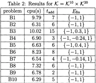
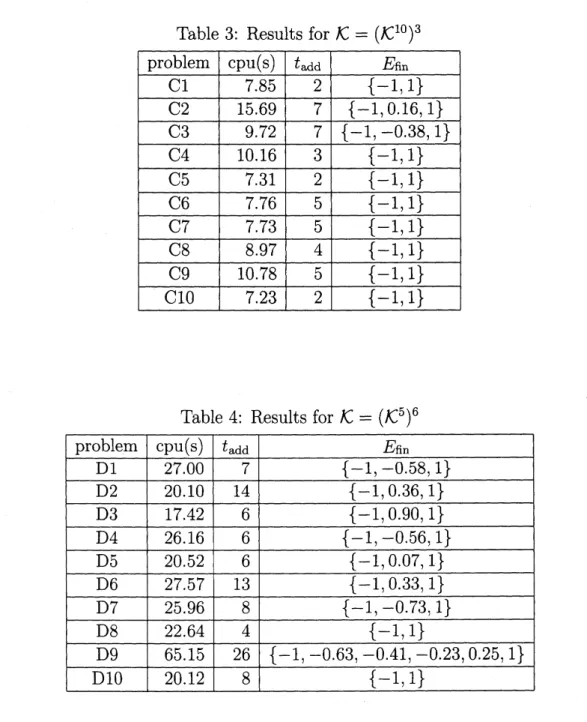
The obtained results

are

shown in Table 1, Table 2, Table 3 and Table 4, in which cpu(s), $t_{add}$ and $Efin$ denote the CPUtime in seconds, the cumulative number

oftimes$t_{new}^{r}$ is added to $T_{r}$ in Step 1, and the value of$E^{k}$ at the termination of the

algorithm, respectively.

From the tables, we can observe that the computational cost tends to be higher

as

the number of

SOCs

in $\mathcal{K}$ gets larger. For example, in the

case

of$\mathcal{K}=\mathcal{K}^{30}$ (one

SOC

in $\mathcal{K})$, the cpu time is only 5 seconds

or

so, whereas it becomes around

20

seconds when $\mathcal{K}=(\mathcal{K}^{5})^{6}$ (six

SOCs

in $\mathcal{K}$). We also note that both $t=-1$ and 1

the constraints $A(t)^{T}x-b(t)\in \mathcal{K}$ with $t=-1$ and

1

are

both

active at the

optimal

solutions. For the problems with $E_{Rn}=\{-1,1\}$, the values of cpu(s) and $t_{add}$

seem

relatively small. In fact, for such problems, the active sets at the optima

can

often beidentified in a small number ofiterations. On the otherhand, if$Efin$ haselements

other than-l

or

1, then the values

of

cpu(s) and $t_{add}$ tend to be larger. Especially,

problems A4, B3,

C2

and D9 yieldthe largest values among the test problems with

$\mathcal{K}=\mathcal{K}^{30},$ $\mathcal{K}=\mathcal{K}^{10}\cross \mathcal{K}^{20},$ $\mathcal{K}=(\mathcal{K}^{10})^{3}$, and $\mathcal{K}=(\mathcal{K}^{5})^{6}$, respectively. Indeed, for

those four problems, $Efin$ has the third element that could not be identified at

an

early stage of the iterations.

Table 1: Results for $\mathcal{K}=\mathcal{K}^{30}$

Table 3: Results for $\mathcal{K}=(\mathcal{K}^{10})^{3}$

Table 4: Results for $\mathcal{K}=(\mathcal{K}^{5})^{6}$

References

[1] F. Alizadeh and D. Goldfarb. Second-order

cone

programming. Mathematical

Progmmming, 95:3-51, 2003.

[2] M. Fukushima, Z. Q. Luo, and P. Tseng. Smoothing functions for second-order

cone

complementarity problems. SIAM Joumal

on

optimization, 12:436-460,

2001.

[3] M.

A. Goberna

and M.

A.

$L6pez$.

Semi-infinite

Programming: Recent Advances.

[4] G. Gramlich, R. Hettich, and E. W. Sachs. Local convergence of SQP methods insemi-infiniteprogramming.

SIAM

Joumal

on

optimization, 5:641-658, 1995. [5] H.

C.

Lai and

S.-Y.

Wu.

On

linear semi-infinite programming problems.

Nu-merical Functional Analysis and optimization, 13:287-304,

1992.

[6] S. Hayashi, T. Yamaguchi, N. Yamashita, and M. Fukushima. A matrix-splittingmethod for symmetric affine second-order

cone

complementarity prob-lems.

Joumal

_of

Computational and Applied Mathematics, 175:335-353,

2005.

[7]

S.

Hayashi, N. Yamashita, and M. Fukushima. A combined smoothingand reg-ularization method for monotonesecond-order

cone

complementarity problems.

SIAM

Joumal

on

optimization, 15:593-615,

2005.

[8] R. Hettich and K. O. Kortanek. Semi-infinite programming: Theory, methods, and applications.

SIAM

Review, 35:380-429,

1993.

[9] C. Kanzow, I. Ferenczi, and M. Fukushima. On the local convergence of

semis-mooth Newton methods for linear and nonlinear second-order

cone

programs without strict complementarity.

SIAM

Joumal on optimization, 20:297-320,

2009.

[10] H. Kato and M. Fukushima. An SQP-type algorithmfor nonlinear second-order

cone

programs. optimization Letters, 1: 129-144, 2007.

[11]

C.

Ling, L. Qi,

G.

L. Zhou, and S.-Y. Wu. Global convergence of

a

robust smoothing SQPmethodforsemi-infinite programming. Joumal

_of

optimization

Theory and Applications, 129:147-164,

2006.

[12] M. S. Lobo, L. Vandenberghe, S. Boyd, and H. Lebret. Applications of second-order

cone

programming. Linear Algebm and its Applications, 284:193-228,

1998.

[13] M. $L6pez$

and

G. Still. Semi-infinite

programming. European Joumal

of

Oper-ational Research, 180:491-518,

2007.

[14] T. Okuno. A regularized explicit exchange method for semi-infinite programs with

an

infinite number of second-order

cone

constraints. Master$s$ thesis,

De-partmentofAppliedMathematics andPhysics, Graduate School ofInformatics, Kyoto University,

2009.

[15] R. Reemtsen and J. R\"uckmann.

_{Semi-infinite}

progmmming. Kluwer Academic

Publishers, Boston, 1998.

[16]

S.-Y.

Wu and D. H. Li and L. Qi and G. Zhou. An iterative method for

solving KKT system of the

semi-infinte

programming. optimization Methods and Soflware, 20:629-643,

2005.

[17] J. F. Sturm. Using SeDuMi 1.02,

a

MATLAB toolbox for optimization

over

[18] Y. Tanaka, M. Fukushima, and T. Ibaraki. A globally convergent SQP method for semi-infinite nonlinearoptimization. Joumal

_of

Computational and Applied Mathematics, 23:141-153, 1988.

[19] K.

C.

Toh, M.

J.

Todd, and

R.

H. T\"ut\"unc\"u. $SDPT3-a$

MATLAB software

package for semidefinite programming, version 2.1. optimization Methods and Software, 11:545-581, 1999.

[20] H. Yamashita and H. Yabe. A primal-dual interior point method for

nonlin-ear

optimization

over

second-order

cones.

optimization Methods and Software, 24:407-426, 2009.