Hagen-Poiseuille and thermal transpiration flows of a highly rarefied gas (Mathematical Analysis in Fluid and Gas Dynamics)

lDepartment

of Mechanical Engineering and Science, Kyoto University, Kyoto 606-8501, Japan

2Advanced

Research Institute of Fluid Science and Engineering,

Kyoto University, Kyoto 606-8501, Japan

Abstract

Hagen-Poiseuille and

thermal

transpiration flows of

a

highly rarefied

gas

through

a

long circular pipe

are

investigated

on

the basis of the linearized Boltzmann equation for

hard-spheremolecules withthediffuse reflection condition. Thenet

mass

flowsoftheboth

problems in the highlyrarefied regime

are

obtained by

an

iterative approximationmethod

with

an

explicit convergence estimate. The singular behavior of the velocity distribution

functions in that regime is also clarified.

1

Introduction

A flowinduced by

a

pressuregradient (Poiseuille flow) and

a

flow inducedby

a

temperature

gradient (thermaltranspiration, see, e.g., Ref. [9]) are classical andfundamental problems

of

rarefied gas

dynamics, and have beenextensivelystudied by many researchers (see,

e.g.,

Refs.

[1,3, 5-9] and the

references

therein).

In the present study,

we

shall focus on Hagen-Poiseuille and thermal transpiration

flows of a highly rarefied gas through

a

circular pipe, for the purpose of obtaining the

accurate data of the net

mass

flows. In the highly rarefied regime,

an

accurate analysis

of these flows

on

the basis of the (linearized) Boltzmann equation is

a

hard task because

ofthe singular behavior ofthe velocity distribution functions, in addition to the complex

collision operator of the equation. In order to

overcome

these difficulties,

we use an

iterative approximation method with

an

explicitconvergenceestimate, which

was

recently

developed by the authors in Ref. [11] withthe aid ofthe mathematical estimates givenby

Chen et al. [2]. Main advantage of this method is that we can start the iterative process

from

an

initial guess with

an

explicit form that contains the majority of the singularity

in the velocity distribution functions. Moreover, the method gives an estimate

on

the

required numberof iterations to obtain the practical convergedsolution and the behavior

ofthe velocity distribution function at each stage of iteration.

Thepaperisorganized

as

follows. Insection 2,

we

formulatethe problems. In section 3,

we

present

an

iterative approximation method and its explicit

convergence

estimate at

each stage of iteration in the highly rarefied regime. Also,

we

clarify the behavior of

the velocity distribution functions by using the estimate. In section 4,

we

present the

numerical methods based

on

the iterative approximation method. Numerical results

are

2

Problem

and

formulation

Consider a highly rarefied gas in a long pipe with a uniform circular

cross

section. Let

the radius of the pipe be $D$ and the $X_{3}$ axis be parallel to the pipe. The pressure of

the gas is given by $p_{0}(1+c_{P}X_{3}/D)$ and the temperature of the pipe wall is given by

$T_{0}(1+c_{T}X_{3}/D)$ ($c_{P}$ and $c_{T}$ are constants). We investigate the steady gas flows under the

followingassumptions: (i) the behavior ofthe gasisdescribed by the Boltzmannequation

for hard-sphere molecules (the mass ofamolecule is $m$ and the diameter ofa molecule is

$d_{m})$; (ii) the gas molecules are diffusely reflected on the surface of the pipe; and (iii) _{$|c_{P}|$}, $|c_{T}|\ll 1$,

so

that the equation and the boundary condition

can

be linearized _around the

equilibrium state at rest with the pressure $p_{0}$ and the temperature $T_{0}$.

Let

us

denote the molecular velocity by $(2RT_{0})^{1/2}\zeta_{i}$ and the velocity distribution

function

of the gas molecules by $\rho_{0}(2RT_{0})^{-3/2}[E^{1/2}+\phi(x_{i}, \zeta_{i})]E^{1/2}$, where _{$x_{i}=X_{i}/D$},

$\rho_{0}=p_{0}/RT_{0},$ $R$ is the specific gas constant, $\zeta=(\zeta_{i}^{2})^{1/2}$, and $E=\pi^{-3/2}\exp(-\zeta^{2})$. Let

us

denote the density of the gas by $\rho_{0}(1+\sigma)$, the flow velocity by $(2RT_{0})^{1/2}u_{i}$, the

temper-ature by $T_{0}(1+\tau)$, the pressure by $p_{0}(1+P)$_, the stress tensor by$p_{0}(\delta_{ij}+P_{ij})$, and the

heat-flow vector by $p_{0}(2RT_{0})^{1/2}Q_{i}$, where $\delta_{ij}$ is Kronecker $s$ delta. Then, the problem is

described by the

following-boundary

value problem for $\phi$:

$\zeta_{i}\frac{\partial\phi}{\partial x_{i}}=-\frac{\nu(\zeta)}{k}\phi+\frac{1}{k}K(\phi)$,

(1)

$\phi=c_{T}(\zeta^{2}-2)E^{1/2}x_{3}-2\sqrt{\pi}E^{1/2}\int_{\zeta_{i}n_{i}<0}\zeta_{i}n_{i}\phi E^{1/2_{\zeta}}K$ for $\zeta_{i}n_{i}>0,$ $x_{1}^{2}+x_{2}^{2}=1$, (2)

where $(2/3) \int\zeta^{2}\phi E^{1/2}d\zeta=CpX_{3}$ and with

$K( \phi)=\int\kappa(\zeta_{i*}, \zeta_{i})\phi(x_{i}, \zeta_{i*})d\zeta_{*}$, (3)

$\kappa(\zeta_{i*}, \zeta_{i})=\frac{1}{\sqrt{2}\pi}\frac{1}{|\zeta_{i}-\zeta_{i*}|}\exp(-\frac{(|\zeta_{i*}|^{2}-|\zeta_{i}|^{2})^{2}}{4|\zeta_{i*}-\zeta_{i}|^{2}}-\frac{|\zeta_{i*}-\zeta_{i}|^{2}}{4})$ $- \frac{1}{2\sqrt{2}\pi}|\zeta_{i}-\zeta_{i*}|\exp(-\frac{|\zeta_{i*}|^{2}+|\zeta_{i}|^{2}}{2})$ , (4) $\int$ノ$( \zeta)=\frac{1}{2\sqrt{2}}[\exp(-\zeta^{2})+(2\zeta+\frac{1}{\zeta})\int_{0}^{\zeta}\exp(-s^{2})ds]$ , (5) $k= \frac{\sqrt{\pi}}{2}\frac{l_{0}}{D}$, $l_{0}= \frac{1}{\sqrt{2}\pi d_{m}^{2}(\rho_{0}/m)}$. (6)

Here, $n_{i}$ is the unit normal vector to the boundary, pointed to the gas and $l_{0}$ is the mean

free path of the gas molecules in the equilibrium state at rest. Note that

we

shall

use

$k$

in place of the Knudsen number Kn $(=l_{0}/D)$ to indicate the degree ofgas rarefaction.

Let

us

introduce the cylindrical coordinate system $(r, \theta, x_{3})$ and $(\eta, \alpha, w)$ in position

and molecular velocityspaces: $x_{1}=r\cos\theta,$ $x_{2}=r\sin\theta,$ $\zeta_{1}=\eta\cos(\theta+\alpha),$ $\zeta_{2}=\eta\sin(\theta+\alpha)$, $\zeta_{3}=w$ (see figure 1). $\eta$ is the absolute value of the molecular velocity in $\zeta_{1}-\zeta_{2}$ plane.

Assuming

the axisymmetry about the $x_{3}$-axis, we can seek $\phi$ in the form of

$\phi=c_{P}[Fx_{3}+\phi_{P}(r, \eta, \alpha, w)]+c_{T}[(\eta^{2}+w^{2}-5/2)Fx_{3}+\phi_{T}(r, \eta, \alpha, w)]$ _{, (7)}

$F= \pi^{-3/4}\exp(-\frac{\eta^{2}+w^{2}}{2})$_,

Fig. 1: Cylindrical coordinate system.

where $\phi_{J}$ $(J=P$

or

T$)$ is the solution ofthe following boundary-value problem:

$\eta\cos\alpha\frac{\partial\phi_{J}}{\partial r}-\frac{\eta\sin\alpha}{r}\frac{\partial\phi_{J}}{\partial\alpha}=-\frac{l\text{ノ}}{k}\phi_{J}+\frac{1}{k}K(\phi_{J})-I_{J}$, (9)

$\phi_{J}=0$ for $\cos\alpha<0,$ $r=1$, (10)

$I_{P}=wF$, $I_{T}=w(\eta^{2}+w^{2}-5/2)F$. (11)

Physically, $\phi_{P}$ represents the solution of the Hagen-Poiseuille flow, while $\phi_{T}$ represents

that of the thermal transpiration. Here

we

have also assumed that $\phi_{J}$ is odd in _$w$ and

symmetric in $\alpha$ in the following

sense:

$\phi_{J}(r, \eta, \alpha, w)=\phi_{J}(r, \eta, 2\pi-\alpha, w)$. (12)

The macroscopic variables

are

expressed

as

$\sigma=(c_{P}-c_{T})x_{3}$, $\tau=c_{T^{X}3}$, $P=c_{pX_{3}}$,

$u_{1}=u_{2}=0$, $u_{3}=c_{P}u[\phi_{P}]+c_{T}u[\phi_{T}]$,

$Q_{1}=Q_{2}=0$, $Q_{3}=c_{P}Q[\phi_{P}]+c_{T}Q[\phi_{T}]$, (13)

$P_{11}=P_{22}=P_{33}=c_{P}x_{3}$, $P_{12}=0$, $P_{23}=- \frac{r}{2}c_{P}\sin\theta$, $P_{31}=- \frac{r}{2}c_{P}\cos\theta$,

where

$u[f]=4 \int_{0}^{\infty}\int_{0}^{\pi}\int_{0}^{\infty}\eta wfFdwd\alpha d\eta$, (14) $Q[f]=4 \int_{0}^{\infty}\int_{0}^{\pi}\int_{0}^{\infty}\eta w(\eta^{2}+w^{2}-\frac{5}{2})fFdwd\alpha d\eta$. (15)

Note that the density, temperature and pressure of the gas

are

uniform in each

cross-section and linearly depend

on

$x_{3}$. The net

mass

flow through the pipe, which

we

denote

by $\rho_{0}(2RT_{0})^{1/2}\pi D^{2}\mathcal{M}$, is written by

3

Iterative approximation method

Integrating Eq. (9) along its characteristic line with the boundary condition (10), we

obtain the following expression for $\phi_{J}$:

$\phi_{J}=\phi_{J}^{(0)}+\int_{0}^{d_{B}}\frac{1}{k\eta}e^{-\frac{\nu}{k\eta}s}K(\phi_{J})_{(\overline{r},\eta,\tilde{\alpha},w)}ds$, (17) $\phi_{J}^{(0)}=-l$ ノ $\underline{k}[1-\exp(-\frac{I\text{ノ}}{k\eta}d_{B})]I_{J}$, (18) with $d_{B}=r\cos\alpha+\sqrt{1-r^{2}\sin^{2}\alpha}$_{, (19a)} $\tilde{r}=\sqrt{r^{2}-2rs\cos\alpha+s^{2}}$_{, (19b)} $\tilde{\alpha}=\cos^{-1}(\frac{r\cos\alpha-s}{\sqrt{r^{2}-2rs\cos\alpha+s^{2}}})$ . (19c)

Here, $d_{B}$is thedistancefrom

$x_{i}$ tothepointonthe boundary in the directionof$(-\zeta_{1}, -\zeta_{2},0)$.

Note that, in Eq. (17), $K(\phi_{J})$ is a function of $\tilde{r}$ and $\tilde{\alpha}$ dependent

on

$s$.

We consider a sequence of functions $\phi_{J}^{(0)},$ $\phi_{J}^{(1)},$ $\phi_{J}^{(2)},$

$\ldots$ generated by the following

iterative process:

$\phi_{J}^{(n)}=\phi_{J}^{(0)}+\int_{0}^{d_{B}}\frac{1}{k\eta}e^{-\frac{\nu}{k\eta}s}K(\phi_{J}^{(n-1)})_{(\overline{r},\eta,\overline{\alpha},w)}ds$

$n=0,1,2,$ $\ldots$, (20)

with $\phi_{J}^{(-1)}=0$. By using the _{mathematical estimates given by}

Chen et al. [2], we

can

prove the following for $k\gg 1$:

(a) $\{\phi_{J}^{(n)}\}$ is a Cauchysequence in

$L^{\infty}$, where the norm is defined by

$||f||_{\infty}= \sup_{\zeta_{i}}|f|$

for each $x_{i}$. The limiting function of$\phi_{J}^{(n)}$ is the solution _{$\phi_{J}:\phi_{J}=\lim_{narrow\infty}\phi_{J}^{(n)}(J=P$}

or

T$)$.

(b) By introducing the sequence of functions $\{\psi_{J}^{(n)}\}$, defined by _{$\psi_{J}^{(n)}=\phi_{J}^{(n)}-\phi_{J}^{(n-1)}$}

$(n\geq 1)$ and$\psi_{J}^{(0)}=\phi_{J}^{(0)},$ $\phi_{J}^{(n)}$ is rewritten

as

$\phi_{J}^{(n)}=\sum_{i=0}^{n}\psi_{J}^{(i)}$. Thus $\phi_{J}$

can

be obtained

as

the sum of$\psi_{J}^{(n)}:\phi_{J}=\sum_{i=0}^{\infty}\psi_{J}^{(i)}$ $(J=P$ or T

$)$. $\psi_{J}^{(n)}$ is generated by the following iterative

process:

$\psi_{J}^{(n)}=\int_{0}^{d_{B}}\frac{1}{k\eta}e^{-\frac{\nu}{k\eta}s}K(\psi_{J}^{(n-1)})_{(\overline{r},\eta,\tilde{\alpha},w)}ds$

$n=1,2,$$\ldots$ . (21)

There

are

positive constants $C_{0}$ and $C_{1}$ independent of $k$ such that, for $i=0,1,$

$\ldots$ ,

$|\psi_{J}^{(i)}|\leq C_{0}(\eta+k^{-1})^{-1}[C_{1}k^{-1}(\ln k+1)]^{i}$_{, (22a)}

$|K(\psi_{J}^{(i)})|\leq C_{0}(1+\ln k)[C_{1}k^{-1}(\ln k+1)]^{i}$_{, (22b)}

$|M[\psi_{J}^{(i)}]|\leq C_{0}[C_{1}k^{-1}(\ln k+1)]^{i}$. _(22c)

On the

one

hand, estimate (22c) shows that the net mass flow at each stage of

iter-ation will be decreased with the rate $O(k^{-1}(\ln k+1))$_. As $k$ is increased, the rate will

$0$ $\eta$ $0$ $\eta$ $0$

(a) (b) (c)

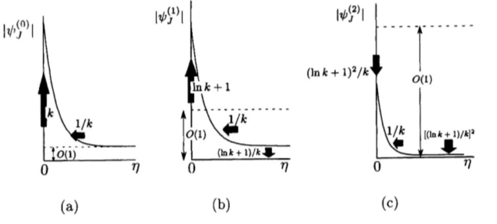
Fig. 2: Change of $\psi_{J}^{(0)},$ $\psi_{J}^{(1)},$ $\psi_{J}^{(2)}$

as

$k$ is increased $(k\gg 1)$. (a) $\psi_{J}^{(0)},$ $(b)\psi_{J}^{(1)},$ $(c)\psi_{J}^{(2)}$.

The rate and direction of change when $k$ is increased

are

shown.

obtained within several iterations. [Actually,

we

needed six iterations for $k=10$ and less

iterations for $k>10$ (see section 5.2).$]$

On

the other hand, estimate (22a) presents that

the velocity distribution function at each stage of iteration will be scaled down with the

rate $o(k^{-1}(\ln k+1))$. We show the feature for $i=0,1,2$ schematically in figure 2. The

figure shows that $\psi_{J}^{(0)}$ will be changed from $o(k)$ to $o(1)$, and $\psi_{J}^{(1)}$ will be changed from

$O(\ln k)$ to $o(1)$ in the range of $o(k^{-1})$ in $\eta$. In other words,

$\psi_{J}^{(0)}$ and $\psi_{J}^{(1)}$ grow locally

near $\eta=0$

as

$k$ is increased. In order to carry out accurate numerical computations for

large $k$,

a

special attention

should

be paidto capturethe singular behavior ofthe velocity

distribution

functions.

4

Numerical method

The net

mass

flowat the initial

guess

$M[\psi_{J}^{(0)}]$, obtainedby substituting$\psi_{J}^{(0)}$ into Eq. (16),

is expressed

as

the forthfold integral. This integral is easily numerically carried out by

first applyingthedouble exponential (DE) transformation [12] to all integration variables

and using the trapezoidal formula for the transformed variables. The number of lattice

points used in this computation is 49 for $r,$ $65$ for $\eta,$ $130$ for $\alpha$ and 97 for $w$ in the ranges

of $0<r<1,0<\eta<4.39,0<\alpha<\pi$ and $0<w<5.93$.

As the first step to obtain higher order corrections $\psi_{J}^{(n)}(n\geq 1)$, by making

use

ofthe

iterative process (21),

we

seek $K(\psi_{J}^{(n-1)})$. In the computation, there

are

two things that

should be paid attention to. One is the fact that $\psi_{J}^{(0)}$ and $\psi_{J}^{(1)}$ behave steeply

near

_$\eta=0$,

as seen

from estimate (22a). The other is the singularity $|\zeta_{i}-\zeta_{i*}|^{-1}$ in Eq. (4). In order

to

overcome

these difficulties,

we

first make the variable transformation from $(\eta_{*}, \alpha_{*}, w_{*})$

to $(P, \beta, w_{*})$ to manage the singularity $|\underline{\zeta_{i}}-\zeta_{i*}|^{-1}$ (see Appendix A). Due to the variable

transformation, in the computation of $L_{1}$,

we

have to capture the singular behavior of

the velocitydistribution function on the transformed coordinate system $(P, \beta, w_{*})$. From

the definition of $\eta_{*}$ [see Eq. (33)],

we

find that $\eta_{*}=0$ corresponds to $P=0,$ $P=\eta$,

$\beta=0,$ $\beta=\pi$and $\beta=2\pi$

on

the transformedsystem for arbitrary $\eta$. Taking into account

this information,

we

divide the domain ofthe integration in such

a

way that $0<P<\eta$

function will be localized

near

the end points of the domains of integrations. The DE

transformation

with the trapezoidal formula is

an

efficient numerical integration method

for an integrand with

an

end-point singularity. By using the DE transformation, $\underline{w}e$

can

$\underline{n}umerically$ handle the $sing\underline{ul}ar$ behavior of the velocity distribution function in $L_{1}$ and $L_{2}$ without difficulties. For $L_{2}$, we do not need to divide the domain of the integration

because the velocity distributionfunction is already localizednear the end-point $(\eta_{*}=0)$.

In the computation of $\overline{L}_{1}$, we give

an additional care in the

case

of $r=1$, because

$\psi_{J}^{(n-1)}$ has discontinuity at _{$\alpha=\pi/2$} (for example,

see

(c) and (f) of figure 3).

As

to

the integration with respect to $s$ in Eq. (21),

we

first interpolate $K(\psi_{J}^{(n-1)})$

for

$\tilde{r}$ and $\tilde{\alpha}$

[see Eqs. (19b) and $(19c)$] because the obtained $K(\psi_{J}^{(n-1)})$ is

a

function of

$r,$ $\eta,$ $\alpha$ and

$w$. After the interpolation, $K(\psi_{J}^{(n-1)})$

can

be approximated by the piecewise quadratic

function on the lattice points of $s$. Thus, the integral of the approximated $K(\psi_{J}^{(n-1)})$

multiplied by exp$(-\iota$ノ$s/k\eta)$ is carried out analytically. We numerically calculate $M[\psi_{J}^{(n)}]$

expressed as the forthfold integral. The integration with respect to $r$ is carried out by

using theSimpson formula, and the integrations with respect to $\eta,$ $\alpha$ and $w$

are

performed

by the trapezoidal formula after the DE transformation.

5

Numerical

results

In

our

computation, themolecular velocity space is limited to $0<\eta<4.39,0<w<5.93$.

The number of lattice points used in the computation ofhigher order correctionsis 21 for

$r,$ $65$ for $\eta,$ $130$ for $\alpha(0<\alpha<\pi)$ and 97 for _$w$.

5.1

Velocity distribution functions

The initial guess $\psi_{T}^{(0)}$, the initial collision operator _{$K(\psi_{T}^{(0)})$}

and the first correction $\psi_{T}^{(1)}$

$hand,\psi_{T}isO(k)and\psi_{T}^{(1)}isO(\ln k+l)Bothofthemare1oca1izedintheregionofatthree\delta_{)}^{ointsinthegasregionareshown.f\circ rk=l0and10^{2}infigures3-5.Ontheone}$

$\eta\leq k^{-1}$. On the other hand, $K(\psi_{T}^{(0)})$, which is _{$o(\ln k+1)$}, behaves moderately in

$\eta$. In

other words, the trace of the singular behavior of$\psi_{T}^{(0)}$ is disappeared in $K(\psi_{T}^{(0)})$. That is,

the singular behavior of $\psi_{T}^{(0)}$

is disappeared by the action of the collision operator with

scaling down by the factor $O(k^{-1}(\ln k+1))$. Bythe actionof the integration_{in Eq. (21),}

a

singular distribution is reproduced in $\psi_{T}^{(1)}$ with

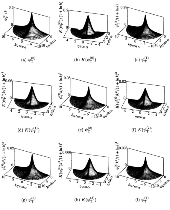
the scale unchanged. We

can

observe the

process of_{disappearance and reproduction of singular velocity distributions in the longer}

transition from $\psi_{T}^{(0)}$ to $\psi_{T}^{(4)}$ at

$r=0$ for $k=10$ in figure

6.

Estimates $(22a)-(22c)$ _may

not be optimal, but the numerical results shown in figures 3-6 support that the estimates

are

actually optimal.

5.2

Net

mass

flows

We have obtained the net

mass

flows of the both problems for several values of $k$. The

numerical results of the initialguess $M[\phi_{J}^{(0)}]$, thefirstcorrection $M[\phi_{J}^{(1)}]$ and the converged

solution $M[\phi_{J}^{(n)}]$

are

shown in table 1. Here _{$\phi_{J}^{(n)}=\Sigma_{i=0}^{n}\psi_{J}^{(i)}$}

$(J=P$

_or

_T$)$. The value of

$M[\phi_{J}^{(n)}]$ is converged to 4 digits. $M[\phi_{J}^{(n)}]$

versus

_$k$ isshown in figure

(a) $k=10,$ $r=0$ (b) $k=10$

.

$r=0.5$ (c) $k=10,$ $r=1$ (d) $k=]0^{2}$. _{$r=0$ (e)} $k=10^{2},$ $r=0.5$ (f) $k=10^{2},$$r=1$ Fig.

3:

$’\psi_{T}^{(0)}$ at $w=0.633$

.

(a) $k=10,$ $r=0$ (b) $k=10,$ $r=0.5$ (c) $k=10,$ $r=1$ (d) $k=10^{2}$

.

_$r=0$ (e) $k=10^{2},$ $r=0.5$ (f) $k=10^{2},$ $r=1$ Fig. 4: $K(\psi_{T}^{(0)})$ at $w=0.633$

.

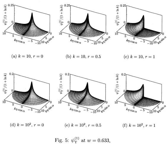
(a) $k=10,$ $r=0$ (b) $k=10,$ $r=0.5$ (c) $k=10,$ $r=1$

(d) $k=10^{2}$. _{$r=0$ (e)} $k=10^{2}$. _{$r=0.5$ (f)} $k=10^{2},$ _$r=1$

Fig. 5: $\psi_{I’}^{(?)}$ at $w=0.633$

.

Finally, welist

some

data that show the accuracy of our computation as follows:

(i) We have limited the molecular velocityspaceto a finiteregion. Inthe computation,

$|\phi_{J}^{(n)}F|$ is less than _{$3.0\cross 10^{-9}$} outside the region.

(ii) The collision integral $K(\phi)-t$ノ$\phi$ for the Maxwellian $\phi=F$ , which should

theo-retically be zero, is bounded by $5.0\cross 10^{-7}$. _{lノ $F$} is of the order of0.3.

(iii) The following moment, which should theoretically be zero, is bounded by

$| \int_{0}^{\infty}\int_{0}^{\pi}\int_{0}^{\infty}\eta w[K(\phi_{J})-\nu\phi_{J}]Fdwd\alpha d\eta|\leq 5.0\cross 10^{-6}$. (23)

6

Conclusion

We have investigated Hagen-Poiseuille andthermaltranspirationflows ofahighlyrarefied

gas through a circular pipe for purpose of obtaining the accurate net

mass

flows. In the

present _{work, motivated by the previous work by the authors, wehave applied}

_an

_iterative

approximation method with

an

explicit

convergence

estimate to the problems, and have

clarified the singular behavior of the velocity distribution function. By making

use

of

the method, with

a

special attention to the singular behavior of the velocity distribution

(a) $\psi_{T}^{(0)}$ (b) $K(\psi_{T}^{(0)})$ (c) $\acute\sqrt{}$_ノ$T(1)$

(d) $K(\psi_{1^{\backslash }}^{(1)})$ (e) $\psi_{1^{\backslash }}^{(2)}$ (f) $K(\psi_{r}^{(2)})$

(g) $\psi_{T}^{(3)}$ (h) $K(\psi_{\Gamma}^{(3)})$ (i) $\psi_{T}^{(4)}$

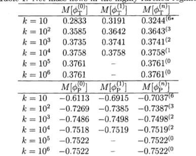
Table 1: Net

mass

flows in the highly rarefied regime. $k=10^{2}$ 0.3585 0.3642 $0.3643^{(3}$ $k=10^{3}$ 0.3735 0.3741 $0.3741^{(2}$ $k=10^{4}$ 0.3758 0.3758 $0.3758^{(1}$ $k=10^{5}$

0.3761

$-$ $0.3761^{(0}$ $k=10^{6}$

0.3761

$0.3761^{(0}$ $\overline{\frac{M[\phi_{P}^{(0)}]M[\phi_{P}^{(1)}]M[\phi_{P}^{(n)}]-}{k=10-0.6113-0.6915-0.7037^{(6}}}$ $k=10^{2}$ _{$-0.7269$ $-0.7385$} $-0.7387^{(3}$ $k=10^{3}$ _{$-0.7486$ $-0.7498$} $-0.7498^{(2}$ $k=10^{4}$ _{$-0.7518$ $-0.7519$} $-0.7519^{(2}$ $k=10^{5}$ _$-0.7522$ $-$ $-0.7522^{(0}$ $k=10^{6}$ _$-0.7522$ $-0.7522^{(0}$

*Converged data.

$T\overline{he}$

superscript number $indicates-$ the order of approximation $n$.

Fig. 7: Net

mass

flows

as

a function of $k$

.

Left figure shows $M[\phi_{T}]$

versus

$k$ and right

figure shows $M[\phi_{P}]$

versus

$k$. $\blacksquare$ indicates the present data.

Appendix A

Collision

operator

$K$

The collision operator $K(\phi_{J})$ is written in the following form:

$K(\phi_{J})=\overline{L}_{1}(\phi_{J})-\overline{L}_{2}(\phi_{J})$, (24)

where

$\overline{L}_{1}(\phi_{J})=\int_{0}^{\infty}\int_{0}^{2\pi}\int_{-\infty}^{\infty}\frac{1}{\sqrt{2}\pi}\frac{\eta_{*}}{|\zeta_{i*}-\zeta_{i}|}\exp(-\frac{(\eta_{*}^{2}+w_{*}^{2}-\eta^{2}-w^{2})^{2}}{4|\zeta_{i*}-\zeta_{i}|^{2}}-\frac{|\zeta_{i*}-\zeta_{i}|^{2}}{4})$

$\cross\phi_{J}(r, \eta_{*}, \alpha_{*}, w_{*})dw_{*}d\alpha_{*}d\eta_{*}$, (25)

$\overline{L}_{2}(\phi_{J})=\int_{0}^{\infty}\int_{0}^{2\pi}\int_{-\infty}^{\infty}\Omega_{2}(\eta, \alpha, w, \eta_{*}, \alpha_{*}, w_{*})\phi_{J}(r, \eta_{*}, \alpha_{*}, w_{*})dw_{*}d\alpha_{*}d\eta_{*}$ , (26)

$\Omega_{2}(\eta, \alpha, w, \eta_{*}, \alpha_{*}, w_{*})=\frac{\eta_{*}}{2\sqrt{2}\pi}|\zeta_{i*}-\zeta_{i}|\exp(-\frac{\eta_{*}^{2}+w_{*}^{2}+\eta^{2}+w^{2}}{2})$ , (27)

$|\zeta_{i*}-\zeta_{i}|=[P^{2}+(w_{*}-w)^{2}]^{1/2}$. (30)

Using Eqs. (29) and (30) in Eq. (25),

we

have

$\overline{L}_{1}(\phi_{J})=\int_{0}^{\infty}\int_{0}^{2\pi}\int_{-\infty}^{\infty}\Omega_{1}(\eta, w, P, \beta, w_{*})\phi_{J}(r, \eta_{*}(\eta, P, \beta), \alpha_{*}(\eta, \alpha, P, \beta), w_{*})dw_{*}d\beta dP$,

(31)

$\Omega_{1}(\eta, w, P, \beta, w_{*})=\frac{1}{\sqrt{2}\pi}\frac{P}{[P^{2}+(w_{*}-w)^{2}]^{1/2}}$

$\cross\exp(-\frac{(P^{2}+2\eta P\cos\beta+w_{*}^{2}-w^{2})^{2}}{4[P^{2}+(w_{*}-w)^{2}]}-\frac{P^{2}+(w_{*}-w)^{2}}{4})$ , (32) $\eta_{*}(\eta, P, \beta)=(P^{2}+\eta^{2}+2\eta P\cos\beta)^{1/2}$, (33)

$\alpha_{*}(\eta, \alpha, P, \beta)=\alpha+\cos^{-1}(\frac{\eta+P\cos\beta}{(P^{2}+\eta^{2}+2P\eta\cos\beta)^{1/2}})$ for $0<\beta<\pi$, (34) $\alpha_{*}(\eta, \alpha, P, \beta)=2\pi+\alpha-\cos^{-1}(\frac{\eta+P\cos\beta}{(P^{2}+\eta^{2}+2P\eta\cos\beta)^{1/2}})$ for $\pi<\beta<2\pi$. (35)

Here, $\eta_{*}\cos(\alpha_{*}-\alpha)=\eta+P\cos\beta$ and $\eta_{*}\sin(\alpha_{*}-\alpha)=P\sin\beta$. Thus, $0<\alpha_{*}-\alpha<\pi$

corresponds to $0<\beta<\pi$ and $\pi<\alpha_{*}-\alpha<2\pi$ corresponds to $\pi<\beta<2\pi$. That is why

we obtain equations (34) and (35).

The threefold integrals (31) and (26)

are

computed numerically by first applying the

DE transformation and using the trapezoidal formula for the transformed variables.

References

[1] C. Cercignani and F.Sernagiotto, “Cylindrical Poiseuilleflow of a rarefiedgas“, Phys.

Fluids 9, 40-44 (1966).

[2] C. -C. Chen, I. -K. Chen, T. -P. Liu and Y. Sone, “Thermal transpiration for the

linearized Boltzmann equation“, Commun. Pure Appl. Math. 60,

0147-0163

(2007).

[3] T. Doi, “Numerical analysis of the Poiseuilleflow and the thermal transpirationof

a

rarefied gas through a pipe with a rectangular

cross

section based on the linearized

Boltzmann equation for a hard sphere molecular gas”, J. Vac. Sci. Technol. A 28,

603-612 (2010).

[4] H. Grad, (Asymptotic theory of the Boltzmann equation, II”, In

_Rarefied

Gas

[5] S.K. Loyalka, “Thermal transpiration in

a

cylindrical tube“, Phys. Fluids 12,

2301-2305 (1969).

[6] S.K. Loyalka and S.A. Hamoodi, “Poiseuille flow of a rarefied gas in a cylindrical

tube: Solution of linearized Boltzmann equation“, Phys. Fluids A 2,

2061-2065

(1990).

[7] G.A. Radtke, N.G. Hadjiconstantinouand W. Wagner, (Low-noiseMonte Carlo

sim-ulation of the variable hard sphere gas“, Phys. Flnids 23 (2011).

[8] C.E. Siewert, “Poiseuille and thermal-creep flow in a cylindrical tube”, J. Co7np.

Phys. 160,

470-480

(2000).

[9] Y. Sone, Molecular Gas Dynamics, Birkh\"auser, (2007).

[10] Y. Sone, T. Ohwadaand K. Aoki, (Temperaturejumpand Knudsen layer ina rarefied

gas

over

a _{plane wall: Numerical analysis of the linearized Boltzmann equation for}

hard-sphere molecules”, Phys. Flui(ls _{A 1, (1989).}

[11]

S.

Takata and H. Funagane, “Poiseuille and thermal transpiration flows of

a

highly

rarefied gas: over-concentration in the velocity distribution function”, J. Fluid Mech.

669, (2011).

[12] H. Takahasi and M. Mori, “Double exponential formulas for numerical integration“,