Random
Strained-Vortices
の統計法則東大・理 畠山望、神部勉
Statistical
Laws
of Random Strained-Vortices in Turbulence
Nozomu Hatakeyama and Tsutomu Kambe
Department
of
Physics, Universityof
Tokyo, Hongo, Bunkyo-ku, Tokyo 113, JapanAbstract
Statistical properties of random distribution of strained vortices (Burgers
vortices) in turbulence are studied, and the scaling behaviors of structure
functions are investigated. It is found within the scale-range of interest
(cor-responding to the inertial range) that the third-order structure function is
negative and the scfflng exponent is nearly unityin accordance with the
Kol-mogorov’sfour-fifths law. The inertial-range scaling exponents are estimated
up to the $25\mathrm{t}\mathrm{h}-_{\mathrm{o}\mathrm{r}\mathrm{d}}\mathrm{e}\mathrm{r}$ which are
in good agreement with those obtained from
experiments and direct numerical simulations once the probability
distribu-tion of the vortex strength is taken into account.
In recent computer simulations and experiments of homogeneous isotropic turbulence at
high Reynolds numbers, a number of elongated intense vortex structures are observed to
distribute randomly in space, which are often called worms [1-5]. Each worm-structure is
found approximately to be a Burgers’ vortex under local straining and is responsible for the
signals usually referred to as the intermittency [5]. Bearing these in mind, we investigate
the statistical properties of a model field associated with random distribution of Burgers
vortices.
High Reynolds numberflows are characterizedbythe statistical properties of the velocity
field $v(x)$ and the difference at two points$x$ and$x+s:\triangle v(x, S)=v(x+s)-v(x)$
.
Definingthe longitudinal difference in the direction $s$ by
$\triangle v_{\ell}(x, s)=\triangle v(x, S)\cdot\frac{s}{s}$ (1)
where $s=|s|$, the $p\mathrm{t}\mathrm{h}$-order longitudinal structure function $S_{p}$ is given by $S_{p}=((\triangle v_{l})^{p})$,
where $\langle$ $\cdot)$ is an ensemble average for a fixed $s$
.
In the homogeneous isotropic turbulence,the structure function $S_{p}$ follows a power-law in the inertial range of$s$:
$S_{p}(s)\equiv((\Delta vl(x, S))^{p})\sim s^{\zeta_{P}}$ (2)
where $\zeta_{p}$ is the scaling exponent of thep-th order structure function.
The skewness $S_{3}/(S_{2})^{3/2}$ in turbulence is always found to be negative for small $s$
.
Theof the velocity derivatives [7]. An example ofa vortex under external straining (considered
below) has such negative skewness. In particular, the third-order structure function is
described by the Kolmogorov’s four-fifths law $[8,9]$,
$\langle(\Delta v_{\ell})^{3}\rangle=-\frac{4}{5}\mathcal{E}S=-\frac{4}{5}\nu\overline{\omega}^{2}S$ (3)
for the values of $s$ in the inertial-range, where the rate of energy dissipation $\epsilon$ is replaced
by an equivalent form $\epsilon=\nu\overline{\omega}^{2},\overline{\omega}$being the $rms$ vorticity. The parameter $\epsilon$ may betermed
more appropriately as the energy transfer across a wave number in the inertial range. In
the Kolmogorov 1941 theory [10], the average ($|\triangle v\ell|\rangle$ at the scale $s$ in the inertial range
is given by dimensional arguments as $\langle|\triangle v\ell|\rangle\sim(\epsilon s)1/3$, and in general the exponent $(_{p}$ is
represented as $\zeta_{p}=p/3$ (referred to as K41 below).
According to thescenarioof Kambe and Hosokawa [11], the present analysis aims at
clar-ifying statistical properties of a mathematical model endowed with a characteristic of the isotropic homogeneous turbulence, namely a random system of strained vortices. This
ap-proach is consistent with the idea of the multifractal model of turbulence field. It is assumed
that, in the limit of large Reynolds number, there is an invariant measure of the
Navier-Stokes turbulence, for which a probability distributionfunction $P(s, \triangle v_{l})$ is defined [9]. The
$p\mathrm{t}\mathrm{h}$-order structure function $S_{p}$ is expressed as an integral $S_{p}(s)= \int(\triangle v_{l})^{p}P(S, \triangle vf)d\triangle v\ell$,
which leads to a power-law in a certain interval of$s$ corresponding to the inertial range, as
actually obtained for the present model below.
Recently aphenomenological step is advanced [12-14]. This is a statistical model taking
account of a hierarchy of fluctuating vortex-filament structures which is found to have
prop-erties of the $log$-Poisson statistics. The resulting exponent of the p-th structure function is
given as $\zeta_{p}=p/9+2-2(2/3)^{p/3}$, which is found to be not far from the direct numerical
simulation(DNS) [1] and the experimental observation $[15,16]$.
Turbulence is regarded as afield of rate-of-strains. At each point, threeprincipal rates of
strain $\alpha,$ $\beta$ and $\gamma$ are defined, andthey satisfy therelation $\alpha+\beta+\gamma=0$ by thesolenoidality
of the velocity field. Assuming the property $\alpha\geq\beta\geq\gamma$, we have always $\alpha\geq 0$ and $\gamma\leq 0$.
The intermediate eigenvalue $\beta$ takes either a positive or a negativevalue.
We consider a velocity field of a strained vortex. The vorticity distribution is assumed
to have only the axial component $\omega(r)$ in the cylindrical coordinate system $(r,\theta, z)$
.
Hencethe vorticity vector is $\omega=(0, \mathrm{O},\omega(r))$ with the axial component $\omega(r)$ specified later. The
velocity associated with $\omega$ is $v_{\omega}=(0, v_{\theta}(r),$$0)$, having only the azimuthal component $v_{\theta}(r)$
.
Thisvortex isexposed to anirrotational straining field given by$v_{\mathrm{e}}=(-ar, 0,2az)$ satisfying
the solenoidal property. The total flow field $v$ is the superposition of $v_{\omega}$ and $v_{\mathrm{e}}$:
$v(x)=(-ar,v_{\theta}(\Gamma),2az)$ (4)
Local principal rates of strain $e_{1},$ $e_{2}$ and $e_{3}$ of the velocity field $v(x)$ are readily calculated
as $e_{1}=-a+|e_{\mathrm{r}\theta}|,$ $e_{2}=2a$ and $e_{3}=-a-|e_{\mathrm{r}\theta}|$, where $e_{\mathrm{r}\theta}=(v_{\theta}’(r)-r-1v\theta(r))/2$. If $|a|$ is
sufficiently small compared with $|e_{\mathrm{r}\theta}|$, then $\alpha=e_{1},$ $\beta=e_{2}$ and
$\gamma=e_{3}$. In the following, the
parameter $a$ is assumed to be positive.
In this circumstance, it can be shown [17] that, with an arbitrary initial axisymmetric
distribution, the axial vorticity $\omega(r)$ (only non-zero-component) tends to the final steady
$\omega_{B}(r)=\frac{\Gamma}{\pi r_{\mathrm{b}}^{2}}\exp(-\hat{\Gamma}^{2})$, $v_{\theta}(r)= \frac{\Gamma}{2\pi r_{\mathrm{b}}}\frac{1-\exp(-\hat{r}^{2})}{\hat{r}}$, (5)
where $\hat{r}=r/r_{\mathrm{b}},$ $r_{\mathrm{b}}=(2\nu/a)^{1/2}$ and $\Gamma$ is the strength. This is the Burgers vortex of
radius
$r_{\mathrm{b}}[18]$ (Fig. 1).
The vortex axes are randomly oriented spatially in isotropic turbulence. In the present
single-worm case, the average is taken over a sphere centered at a chosen reference point
$x$. For example, local third-order moment $\hat{s}_{3}=\langle(\partial v_{I}/\partial s)^{3}\rangle_{\mathrm{s}_{\mathrm{P}}}|_{s=0}$ (skewness without
nor-malization) of the longitudinal derivative at $x$ is calculated $[19,20]$ as $\hat{s}_{3}=(8/35)e_{1}e_{2}e_{3}=$
$-(16/35)a(e_{\mathrm{r}\theta}^{2}-a)2$, where the spherical average $\langle\cdot\rangle_{\mathrm{s}\mathrm{p}}$ is an integral over the solid angle
with respect to the direction $s$ divided by $4\pi$
.
It is found that for a pure vortex$v_{(v}$ without
any external strain (hence $a=0$), $\hat{s}_{3}$ is zero, while the converse case of a pure straining
$v_{\mathrm{e}}$ without the vortex (thus $e_{\mathrm{r}\theta}=0$), $\hat{\mathit{8}}3=$ (16/35) $a^{3}$ is positive. However, the composite
flow field considered above gives a negative $\hat{s}_{3}$ as far as $|e_{\mathrm{r}\theta}|>a$
.
Therefore the spacesur-rounding the intense vortex under the straining of$v_{\mathrm{e}}$ is characterized as a field of negative
skewness. Local rate of energy dissipation is given as $\dot{\epsilon}_{1_{\mathrm{o}\mathrm{C}}}(r)=\nu\{12a^{2}+(2e_{\mathrm{r}\theta})2\}$, where
$2e_{\mathrm{r}\theta}\equiv v_{\theta}’(r)-r-1v\theta(r)=(\Gamma/\pi r_{\mathrm{b}}^{2})[\exp(-\hat{r}^{2})-\hat{r}^{-2}(1-\exp(-\hat{r}^{2})]$
.
If $\Gamma/(\pi r_{\mathrm{b}}^{2})$ is sufficientlylarge compared with $a$, the energy is strongly dissipated at around
$r_{\mathrm{b}}$, while at the center
of vortex scarcely dissipated. Taking an average of the local third-order moment over a
spherical surface of radius $s=|s|$, we have $\langle(\Delta v_{\ell})^{3}\rangle_{\mathrm{s}_{\mathrm{P}}}\approx\hat{s}_{3}s^{3}$when $s$ is sufficiently small.
Owing to the solenoidal property of the velocity, the average $\langle\triangle v\ell\rangle \mathrm{s}\mathrm{P}$ vanishes identically.
Next, weinvestigate the behaviors of the longitudinal velocity difference $\triangle v_{I}(s)$ at large
distances, in particular, general$p\mathrm{t}\mathrm{h}$-order structure functions. Fixing a reference point
$x$ at
$(r_{0},0, z_{0})$ in the cylindrical system $\mathrm{K}_{1}$: $(r, \theta, z)$, we define a spherical polar coordinates $\mathrm{K}_{2}$:
($s$,$(, \phi)$ centered at $x$ to represent the relative position of the point $x+s$, where $\zeta$ is the
polar angle and $\phi$ the azimuthal angle. For the velocity field (4) and (5), the longitudinal
velocity difference is represented as
$\triangle v_{\ell}(X, S, \zeta, \phi)=as(3\cos\zeta 2-1)+r_{0}W(r,r0)\sin\zeta\sin\phi$ (6)
where $W(r,r_{0})=r^{-1}v_{\theta}(r)-r-1v_{\theta(r_{0})}0$
.
The spherical average is calculated by$\langle(\triangle v\ell)^{p}\rangle_{\mathrm{s}_{\mathrm{P}}}(x,s)\equiv\frac{1}{4\pi}\int_{-\pi}^{\pi_{d\phi}}\int_{0}\pi\triangle(v\ell)p\mathrm{i}\mathrm{s}\mathrm{n}\zeta d\zeta$ . (7)
Thisaverage will depend on thepoint $x$ as well as the separation vector $s$ andhave different
scaling behaviorswith respect to $s$ at different$x’ \mathrm{s}$ inaccordance with the multifractalaspect.
The statistical average $\langle\cdot\rangle$ is taken firstly by the spherical average
$\langle\cdot\rangle_{\mathrm{s}\mathrm{p}}\mathrm{w}\mathrm{i}\dot{\mathrm{t}}\mathrm{h}$respect to
the running point $x+s$, and secondlyby volume average with respect to the reference point
$x$:
$\langle\cdot\rangle(S)=\frac{1}{\pi R_{0}^{2}\triangle z}\int_{0}^{\Delta z}dz_{0}\int_{0}^{R_{0}}\langle\cdot)_{\mathrm{s}\mathrm{p}}2Tr0dr0$ (8)
(the average with respect to $z_{0}$ is trivial). Thus we obtain the statistical properties of
isotropy and homogeneity from the velocity field (4).
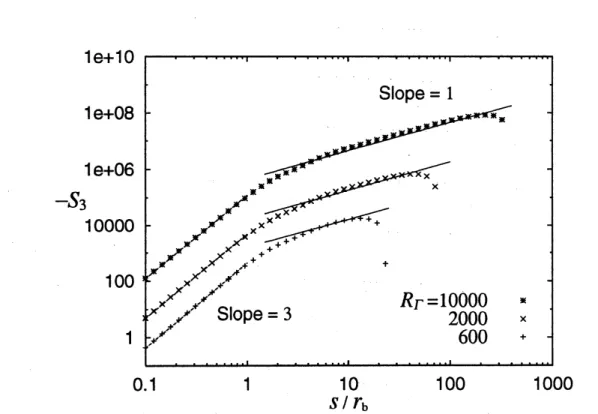
The structure functions are estimated for three different strengths of the Burgers vortex
$S_{3}(s)$ are shown. At small distances $s/r_{\mathrm{b}}<1$, the function $S_{3}(s)$ is proportional to $s^{3}$ as
anticipated for the continuous smooth field. However for $s/r_{\mathrm{b}}>1$ the function $S_{3}(s)$ shifts
to another scaling law of a different slope. It is found that the third-order scaling exponent
$\zeta_{3}$ in the second scaling range is about unity and almost independent of the magnitude of
$R_{\Gamma}$
.
Straight lines with unit slope are obtained from Kolmogorov’s four-fifths law (3), wheremean energy dissipation rate is defined as $\epsilon=(\pi R_{0}^{2})^{-1}\int_{0\mathrm{o}\mathrm{c}}^{R0_{\mathcal{E}_{1}}}(r\mathrm{o})2\pi r_{0}dr_{0}$
.
The limit of$r_{0}$-integral is given by $R_{0}=2.5r_{\mathrm{b}}$ so as to be consistent with the four-fifths law for the
second scaling range. The first scaling range of the exponent 3.0 is identified as the viscous
range, and the second rangeof the exponent 1.0as the inertial rangewhichis wider for larger
$R_{\Gamma}$
.
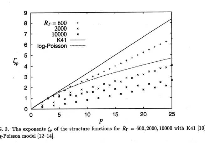
In Fig. 3, the scaling exponents $\zeta_{p}$ up to $p=25$ are shown for the three values of $R_{\Gamma}$,and compared with those of $\mathrm{K}41$ and $\log$-Poisson model. Increasing the magnitude $R_{\Gamma}$, the
exponents $(_{p}$ decreasemore below the K41. The even-p exponents fall lower than the line of
the odd-p exponents, which is in agreement with the general behavior of the experimental
data [15].
The probabilitydistribution functions of the vortex Reynolds number $R_{\Gamma}$ and the
Burg-ers’radius $r_{\mathrm{b}}$ in turbulence are estimated by Jimen\’ez et al. [2] in DNS and by Belin et al. [5]
experimentally. In particular, distributions of the normalized values $R_{\Gamma}/R_{\lambda^{/2}}^{1}$ are
indepen-dent of the valueofthe Reynolds number $R_{\lambda}$ based on the Taylor microscale $\lambda$. Taking into
account of the probability distribution, the structure functions are estimated [21].
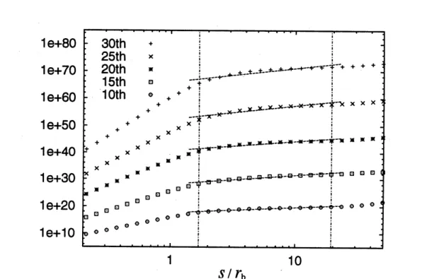
In Fig. 4 and Fig. 5, behaviors of such structure functions are illustrated. It is observed
that there exist two scaling ranges in each structure function, in which the second one
corresponds to the inertial range. Here the inertial range is defined as the range within
which the variance of the third-order structure function with respect to the four-fifth law
is least. In Fig. 6, the scaling exponents in the inertial range are plotted and compared
with those obtained from other models, DNS and experiments. It is found that the present
analysis can predict the scaling exponents which are remarkably coincident with those of
DNS [1] and the experiments $[15,16]$
.
If the vortex is absent (therefore $v_{\theta}=0$), we have $S_{p}(s)=C_{p}a^{p_{S}p}\propto s^{p}$ from Eq. (6)
and Eq. (7), where $C_{p}$ is a constant. On the other hand, if the external strain is absent
(therefore $a=0$), we find that the structure functions of the odd-order are identically zero
by the antisymmetric property of Eq. (6). Hence the present scaling exponents consistent
with the homogeneous isotropic turbulence have resulted from the combined field of the
vortex and the turbulence straining.
The present study is summarized as follows.
1. It is found from the velocity field of random distribution of Burgers vortices that
the third-order structure function is negative in the inertial range and the scaling
exponent is nearly unity and independent of the vortex Reynolds number $R_{\Gamma}$, and
that the second-order structure function has the scaling exponent of about two-thirds,
in accordance with the general turbulence properties.
2. Thescaling exponents of the high-order structure functions deviate increasingly below
K41 as $R_{\Gamma}$ becomes larger. A Burgers vortex in turbulence causes more and more the
3. The scaling exponents $\zeta_{p}$ are in good agreement with the experiments and DNS data
once the distribution function of $R_{\Gamma}$ (takenfrom the experiments and DNS) is taken
REFERENCES
[1] A. Vincent and M. Meneguzzi, J. Fluid Mech. 225, 1 (1991).
[2] J. Jimen\’ez, A. A. Wray, P. G. Saffman, and R. S. Rogallo, J. Fluid Mech. 255, 65
(1993); J. Jimen\’ez and A. A. Wray, CTR Annual Res. Briefs, 287 (1994).
[3] H. Yamaguchi, S. Oide, K. Yamamoto, and I. Hosokawa, in The 9-th Symp. on Comp.
Fluid Dyn. (1995), pp. 167-168 [in Japanese]; S. Oide, T. Sato, I. Hosokawa, K.
Ya-mamoto, and K. Suematsu, in The 28-th Symp. on Turbulence (1996), pp. 55-56 [in
Japanese].
[4] M. Tanahashi, T. Miyauchi, and T. Yoshida, in The 9-th Symp. on Comp. Fluid Dyn.
(1995), pp. 171-172 [in Japanese]; in The 7-th Symp. on Comp. Fluid Mech. (1996), pp.
189-190 [in Japanese].
[5] F. Belin, J. Maurer, P. Tabeling, and H. Willaime, J. de Phys. II France 6, 573 (1996).
[6] G. K. Batchelor and A. A. Townsend, Proc. Roy. Soc. A 190, 534 (1947).
[7] T. Kambe, Fluid Dyn. Res. 8, 159 (1991).
[8] L. D. Landau and E. M. Lifshitz, Fluid Mechanics (Pergamon, 2nd ed., 1987), \S 34.
[9] U. Frisch, Turbulence (Cambridge U.P., Cambridge, 1995), chap. 6, 8.
[10] A. N. Kolmogorov, C. R. Acad. Sci. USSR 30, 301 (1941); ibid. 32, 16 (1941).
[11] T. Kambe and I. Hosokawa, in Small-Scale Structures in Three-Dimensional
Hydrody-namic and Magnetohidrodynamic Turbulence, edited by M. Meneguzzi, A. Pouquet and
P. L. Sulem (Springer-Verlag, 1995), pp. 123-130.
[12] Z. -S. She and E. Leveque, Phys. Rev. Lett. 72, 336 (1994).
[13] B. Dubrulle, Phys. Rev. Lett. 73, 959 (1994).
[14] Z. -S. She and E. C. Waymire, Phys. Rev. Lett. 74, 262 (1995).
[15] G. Stolovitzky, K. R. Sreenivasan, and A. Juneja, Phys. Rev. E48, 3217 (1993).
[16] F. Belin, P. Tabeling, and H. Willaime, Physica D93,52 (1996).
[17] T. Kambe, J. Phys. Soc. Jpn. 53, 13 (1984).
[18] J. M. Burgers, Adv. in Appl. Mech. 1, 171 (1948).
[19] A. A. Townsend, Proc. Roy. Soc. London A 208, 534 (1951).
[20] D. I. Pullin and P. G. Saffman, Phys. Fluids A 5, 126 (1993).
[21] In order to estimate the mean vortex Reynolds number, it is assumed for isotropic
turbulence that $\sigma=v_{\mathrm{r}\mathrm{m}\mathrm{s}}/\lambda$ and $\Gamma=2\pi r_{\mathrm{b}}v_{\mathrm{r}\mathrm{m}\mathrm{s}}$, where $\sigma$ is the axial stretching rate of
worm ($\sigma=2a$ in case of Burgers’ vortex) and $v_{\mathrm{r}\mathrm{m}\mathrm{s}}$ the $\mathrm{r}\mathrm{o}\mathrm{o}\mathrm{t}- \mathrm{m}\mathrm{e}\mathrm{a}\mathrm{n}-_{\mathrm{S}}\mathrm{q}\mathrm{u}\mathrm{a}\mathrm{r}\mathrm{e}$velocity. The
consequenceis $R_{\Gamma}/R_{\lambda}^{1/2}=4\pi$, in good agreement withthe value obtained by Jimen\’ez et
al. in DNS [2]. Thus the PDF of $R_{\Gamma}$ is defined as $P(R_{\Gamma})=(C^{3}/2)R_{\mathrm{r}^{\mathrm{e}\mathrm{x}}}^{2}\mathrm{p}(-^{cR}\mathrm{r})$ with
C $=(3/4\pi)R_{\lambda}^{1}/2$, so that the mean value of $R_{\Gamma}$ is $4\pi R_{\lambda}^{1/2}$ and the PDF has the similar
FIGURES
FIG. 1. The localenergy dissipation rate$\epsilon_{1\mathrm{o}\mathrm{c}}$, the axial vorticity$\omega_{B}$ andthe azimuthal velocity
$v_{\theta}$ ofthe Burgers’ vortex for $R_{\Gamma}\equiv\Gamma/\nu=2000$ normalized by $\nu=0.1$
.
U.l 1 1U IUU lUUo
$S/\gamma_{\mathrm{b}}$
FIG. 2. The third-order structure functions times $-1$ for $R_{\Gamma}=600$,2000,10000 with $\nu=1$
.
1
$\rceil$ $1\cup$
$S/\gamma_{\mathrm{b}}$
FIG. 4. The first-, second- and third-order structure functions for $R_{\lambda}=$ 2000. The region
between the dotdased lines is regarded as inertial range. Solid line is given by the Kolmogorov’s
four-fifths law (3) with $\epsilon=(\pi R_{0}^{2})-1\int 0\Gamma\infty dR\int_{0}^{R}0\mathcal{E}1\mathrm{o}\mathrm{c}(R_{\Gamma}, r)P(R\mathrm{r})2\pi rdr$, and dashed lines are the
I 1$\mathrm{u}$
$S/\gamma_{\mathrm{b}}$
FIG. 5. High-order structure functions with fitting lines in the inertial rangefor $R_{\lambda}=2000$
.
$\zeta_{p}$
FIG. 6. The exponeni $\zeta p$ oi $\tau \mathrm{n}\mathrm{e}\mathrm{s}\tau \mathrm{r}\mathrm{u}\mathrm{C}\mathrm{t}\mathrm{u}\mathrm{r}\mathrm{e}$Iuncuon Ior $\mathrm{J}\mathrm{t}_{\lambda}=$
zuuu
wltll A41$\lfloor 1\mathrm{U}\rfloor$, log-Poisson
model [12-14], DNS for $R_{\lambda}=200$ by Vincent and Meneguzzi [1], a wind tunnel experiment for
$R_{\lambda}=200$ by Stolovitzky et al., obtained from taking the pollution of viscous range into
ac-count [15], and aheliumgasexperiment for $R_{\lambda}=2000$ by Belin et al., obtained byuseof extended