Doctoral Thesis reviewed
by Ritsumeikan University
Seiberg-Witten Geometry
and
the Nekrasov-type Partition Function
in
E-string Theory
(
E
弦理論におけるサイバーグ
-
ウィッテン幾何学と
ネクラソフ型分配関数)
September, 2015
2015
年
9
月
Doctoral Program in Advanced Mathematics and Physics
Graduate School of Science and Engineering
Ritsumeikan University
立命館大学大学院理工学研究科
基礎理工学専攻博士課程後期課程
ISHII Takenori
石井 健准
Supervisor: Professor SUGAWARA Yuji
Abstract
In this thesis, the E-string theory, that is the interacting, non-gravitational local quantum field theory with (1,0) supersymmetry and the E8global symmetry in six
dimensions, is surveyed. By the toroidal compactification, we can obtain theN = 2 supersymmetric gauge theory in four dimensions. This theory is allowed to have its Seiberg-Witten description. In 2012, the Nekrasov-type partition function for E-string theory appeared. As the original Nekrasov partition function was required the proof of the correctness, the Nekrasov-type partition function also was.“ The proof”is given by extracting the Seiberg-Witten description in the thermodynamic limit from the Nekrasov-type partition function, following the idea by Nekrasov and Okounkov. Due to the toroidal compactification, in E-string theory we obtain an elliptic function on the way to prove. The elliptic function gives the Seiberg-Witten description. The Nekrasov-type partition function is also valid in the cases with the general Wilson lines. Moreover, the Nekrasov-type partition function clarifies the dependence of the Seiberg-Witten curve on the Wilson lines.
Contents
1 Introduction 3
2 Two Prescriptions in 4dN = 2 Gauge Theory 6
2.1 Seiberg-Witten description . . . 6 2.2 Nekrasov partition function . . . 8
3 E-string Theory 13
3.1 Formulation of E-string Theory . . . 14 3.2 Two Prescriptions of E-string Theory . . . 16
4 Nekrasov-type Partition Function For E-string Theory 18
4.1 Proof: Nekrasov and Okounkov approach . . . 20 4.2 The case of E-string theory . . . 25
5 The Generalisation to the Cases with Wilson Lines 30
5.1 The cases with three Wilson lines . . . 30 5.2 The cases with four Wilson lines . . . 36 5.3 The derivation of the S L(3, C) invariant curve . . . 37
6 Examples of the Cases with the Broken Symmetries 41
6.1 E7⊕ A1 . . . 41 6.2 E6⊕ A2 . . . 44 6.3 D8 . . . 47 7 Conclusion 48 A The functionγϵ1,ϵ2(x;Λ) 51 B The notations 52
1
Introduction
String theory is the most reliable model for the study of the fundamental struc-ture of an object. Superstring theory, or simply superstring, is the string theory with supersymmetry. The study of superstring has given not only a lot of physical predictions but also a lot of mathematical predictions. However, there are five different types of superstrings, so we have a big problem: which can describe our physics? However, E. Witten showed that there exists the theory in eleven di-mensions which contains all the superstrings[1]. This eleven-dimensional theory is called M-theory and is expected to be the more fundamental theory. M-theory has membranes as the ingredients which are called an M2- and an M5-brane. One of methods of study of M-theory is to study the worldvolume theory on the M5-brane. The worldvolume theory is the six-dimensional theory and has supersym-metry. The number of supersymmetry depends on the configuration of the M2-and M5-branes. The six-dimensional theory can have three types of the number of supersymmetry and they are called the (2,0), (1,1), and (1,0) theories respec-tively1 . The six-dimensional (2,0) theory is the maximal supersymmetric theory.
Recent years, this theory has been intensively studied and has given a lot of in-teresting results not only in physics but also in mathematics. One of these is the
AGT correspondence[2, 3]. The AGT correspondence relates the Nekrasov
parti-tion funcparti-tion of anN = 2 supersymmetric gauge theory in four dimensions to the conformal block(roughly speaking, the correlation function) of a conformal field theory in two dimensions.
The six-dimensional (1,0) theory is the minimal supersymmetric theory, on the one hand. The six-dimensional (1,0) theory with the least field content, more explicitly just one tensor multiplet, and the E8 global symmetry is called the
E-string theory and this theory is the main subject in this thesis.
The history of E-string theory was started by P. Horava-E. Witten and O. J. Ganor-A. Hanany[4, 5, 6]. Briefly speaking, Horava and Witten showed that in M-theory on S1/Z2each E8gauge field must live on the end-of-the-world
brane(M9-brane) to reproduce the E8× E8 heterotic superstring theory in the small S1/Z2
limit2. Ganor and Hanany showed that, in such a case, in the limit where an
M5-brane between the M9-M5-branes approaches one of the M9-M5-branes, an M2-M5-brane between the M5-brane and the M9-brane becomes a tensionless and non-critical
1We make some comments on the study of the (2,0) and (1,0) theories in Introduction. However
we make no mention of the (1,1) theory here.
2Before the discussion of a small instanton associated to the E
8 × E8 heterotic superstring
string. This string is called the E-string and the theory which describes the
be-haviour of the E-string on the M5-brane is called the E-string theory. We will review this theory in more detail in section 3.
E-string theory is known as the simplest, six-dimensional (1,0) theory. The theory consists of just one tensor multiplet, namely has no gravity. In addition, the theory has the E8 global symmetry. However, the theory does not have its
Lagrangian description at present.
When it comes to the four-dimensional theories, in particular with eight su-percharges, we know a lot. More explicitly, the four-dimensional N = 2 su-persymmetric gauge theories have two major descriptions: the Seiberg-Witten theory[8] and the Nekrasov partition function[11]. Thus in that sense, we can say that the four-dimensional N = 2 supersymmetric gauge theories are the best understood theories. So we would like to move on from the world in six dimen-sions to that in four dimendimen-sions. By taking two dimendimen-sions to be very small in the six-dimensional theories, we can obtain the four-dimensional N = 2 super-symmetric gauge theories and study them. This procedure is called dimensional
reduction. Then to keep supersymmetry, the two dimensions must be a compact
manifold, i.e. R4× M2where M2denotes the two-dimensional compact manifold. This procedure is called compactification. In E-string theory, the two dimensions must be a torus T2because we have to keep the eight supercharges. This is called
the toroidal compactification. By the toroidal compactification, we can obtain the four-dimensional N = 2 supersymmetric gauge theory, but the nature of it is so different from that of the ordinary four-dimensional N = 2 supersymmetric gauge theories[9]. For instance, the four-dimensionalN = 2 supersymmetric gauge the-ory obtained from E-string thethe-ory is asymptotically non-free. More details will be mentioned in section 3. Nevertheless, it was shown that it has the Seiberg-Witten description[9, 10]. Hence, following the history of the four-dimensional
N = 2 supersymmetric gauge theories, namely the discovery of the Nekrasov
partition function several years later since the appearance of the Seiberg-Witten description, it is natural to expect that there also exists the Nekrasov-type par-tition function in E-string theory. The Nekrasov parpar-tition function includes the Seiberg-Witten description as the special limit[11, 12]. Hence it is the very im-portant problem to ask whether the Nekrasov-type partition function in E-string theory exists or not for the development of E-string theory.
From such an expectation, in 2012 the Nekrasov-type partition function was given by K. Sakai[13, 14]. The correctness or the validity of the Nekrasov-type partition function was checked order by order, by comparing the values given by the Nekrasov-type partiton function with the ones given by the partition function
of theN = 4 topological super Yang-Mills theory on 12K3[16] and the ones given by the prepotential. In addition it was also checked that the Nekrasov-type parti-tion funcparti-tion satisfies the holomorphic anomaly equaparti-tion[35]. However,“ order by order ”means“ not all orders. ”Namely, in order for the Nekrasov-type par-tition function to be correct, i.e. it is the formula, that it is correct for all orders has to be shown. The Nekrasov partition function and some statements associated to it were given in [11] and then their correctness was given in the subsequent paper[12]. Hence it is natural to expect that we can show the correctness of the Nekrasov-type partition function for all orders by following the idea of [12]. K. Sakai and the author showed it in [15]. More details will be discussed in section 3.
Briefly speaking, our goal is to show that we can extract the known Seiberg-Witten description in E-string theory from the Nekrasov-type partition function. Following the idea of Nekrasov and Okounkov[12], the Nekrasov-type partition function is represented by some Young diagrams and functions associated to them which are called the profile functions. In the semiclassical limit which is called the thermodynamic limit, we can fix them explicitly. Then in E-string theory, due to the toroidal compactification, the profile functions are fixed by an elliptic function. This elliptic function plays a crucial role in our discussion. Namely, we showed that we can extract the Seiberg-Witten description if we give the elliptic function depending on a case. Here“ case ”means that for the special values of the Wilson lines, the global symmetry would be partially broken.
In the subsequent paper[29], the author generalised the result of [15] to more general cases. Namely, whilst in [15] we studied some cases with the Wilson lines given the concrete values, in [29] the cases with three and four general Wil-son lines were discussed. By the study[29], it was shown that the Nekrasov-type partition function is also valid for the general case and was shown the dependence of the Seiberg-Witten curve on the Wilson lines explicitly. In particular, the lat-ter is inlat-teresting for us. The Seiberg-Witten curve in the case with three general Wilson lines is already known[26]. It was obtained by the so-called geometric
en-gineering approach. However, in that case, the dependence of the Seiberg-Witten
curve on the Wilson lines was not clear. We will comment about this point in Conclusion again.
This thesis is organised as follows. In the next section, we briefly review the Seiberg-Witten description and the Nekrasov partition function. In particular, we will focus on the ideas which we will need for the later discussions. In section 3, we will review the formulation of E-string theory, its Seiberg-Witten description, and the Nekrasov-type partition function. In addition, we will see briefly the
va-lidity, or in other words the interpretation of the Nekrasov-type partition function. In section 4, we will prove the correctness of the Nekrasov-type partition func-tion, i.e. we will show that we can extract the Seiberg-Witten description from the Nekrasov-type partition function. In section 5, the result of section 4 is gener-alised to the cases with the Wilson lines. In section 6, the examples of the cases with the broken symmetries are summarised. Sections 4, 5, and 6 are the original parts based on [15, 29]. Finally, in section 7 we will summarise the stories. In appendix A, the functionγϵ1,ϵ2(x;Λ) which will be used in sections 2 and 4 will be summarised. In appendix B, the definitions and the useful relations of the elliptic functions which will be used in sections 4, 5, and 6 will be summarised.
2
Two Prescriptions in 4d
N = 2 Gauge Theory
In this section, we review the ordinaryN = 2 supersymmetric gauge theory in four dimensions before we move on to our main discussion, that is, the Nekrasov-type partition function for E-string theory. Firstly, we very briefly recall the Seiberg-Witten description for the ordinary theory and E-string theory. And secondly, we briefly review the discussion of the so-called Nekrasov partition function to move on to that for E-string theory.2.1
Seiberg-Witten description
In 1994, N. Seiberg and E. Witten determined the low-energy effective action in theN = 2 supersymmetric gauge theory in four dimensions3[8]. More precisely speaking, they gave the prescription to determine the prepotential of the theory which gives the action(we say Lagrangian alternatively henceforth). Here the
low-energy e f f ective means so-called Wilsonian, that is, by integrating out the
massive modes, we make the theory consist only of the almost massless modes. The low-energy effective Lagrangian of the theory with N = 2 supersymmetry is given by Le f f = 1 8πi ∫ d2θ∂ 2F (Φ) ∂Φ2 W αW α+ 1 4πi ∫ d2θd2θΦ¯ †∂F (Φ) ∂Φ + h.c. (2.1)
whereF denotes the prepotential, Φ(z) the complex scalar superfield, and Wαthe chiral superfield including the vector field. Note, here, that from (2.1) we have the
gauge couplingτ:
τ = ∂2∂ΦF (Φ)2 . (2.2)
The prepotentialF (Φ) is a holomorphic function. Thus determining the holomor-phic function is to give the Lagrangian. The prepotential can be written, byN = 2 supersymmetry, as
Prepotential= classical + 1-loop + non-perturbative. (2.3) In the r.h.s., the first two terms can be determined by the classical discussion as
1 2τcla 2+ i 2πa 2 log( a 2 Λ2 ) , (2.4)
where a denotes the Higgs vev andΛ the so-called QCD dynamical scale.
The long-standing problem was to determine the non-perturbative part. The form was known as
∞ ∑ k=1 Fk(Λ a )4k a2. (2.5)
This is known as the so-called instanton expansion, which forms the series by the instanton number k. Seiberg and Witten showed that this can be determined by using the period integrals in algebraic geometry which is known as the moduli theory of torus.
The key ingredients of their discussion are a one-form, two one-cycles, and an elliptic curve, which are called the Seiberg-Witten di f f erential, the α- and
β-cycles, and the Seiberg-Witten curve respectively. For instance, for S U(2), we
give just the result:
aD := ∂F (a) ∂a , ω := I α dz y , ωD:= I β dz y , τ(a) = ∂aD ∂a = ∂aD ∂u ∂u ∂a, 2πi ∂aD ∂u = ω, 2πi ∂a ∂u = ωD, a(u) = I α ds, aD(u)= I β ds, ds = 1 πi z2dz y , y2 = (z2− u)2− 4Λ2 = 2 ∏ i=1 (z− α−i )(z− α+i). (2.6)
Treating the Higgs vev a and its dual aDas functions with respect to the modulus
u := ⟨Trϕ2⟩ = a2/2 is the basic idea. The prepotential is fixed by the beta-cycle
integral of the Seiberg-Witten differential ds. The two cycles are taken by two cuts over [α−1, α+1] and [α−2, α+2]. The period integral or the Seiberg-Witten differential is fixed by the Seiberg-Witten curve y2. The discussion by Seiberg and Witten
states that we are able to determine the prepotential by going up the river.
2.2
Nekrasov partition function
As seen in the last subsection, we can obtain the prepotential by using the acrobatic algebraic geometrically method. However, it is hard to determine the prepoten-tial practically. A few years later, a new approach appeared. It can combina-torially determine the prepotential and what we need is just the field content of the theory. In other words, if we even know the field content, we can directly give the prepotential. More precisely, it gives directly not the prepotential but the
partition f unction. More explicitly, Nekrasov proposed the expression4[11]
Z(⃗a, ϵ1, ϵ2, Λ) = exp ( − Finst(⃗a, ϵ1, ϵ2, Λ) ϵ1ϵ2 ) . (2.7)
The detail including the notation is given later. The important thing is that the partition function Z(⃗a, ϵ1, ϵ2, Λ) and the instanton part of the prepotential Finstare
both generic, that is, they are generalised by the two parametersϵ1,2. So Nekrasov
proposed one more strong relation[11]: in the limit ϵ1,2 → 0, (2.7) would
repro-duce the Seiberg-Witten description, i.e.5
Finst(⃗a, ϵ
1, ϵ2, Λ)|ϵ1,2=0is the instanton part of the prepotential of the low-energy theory.
(2.8) In the rest of this subsection we review the so-called Nekrasov partition
func-tion more detail and pursue the idea of the proof of it, that is, extracting the Seiberg-Witten description.
4The prepotential consists of the perturbative part and the non-perturbative part. Similarly, the
Nekrasov partition function also consists of the perturbative part and the non-perturbative part. In this thesis, we restrict ourselves to the non-perturbative part, i.e. the instanton part. In the sense, by the Nekrasov partition function Z we mean the instanton partition function of the full partition function.
From now on, we also consider the Nekrasov partition function in the field the-oretic limit, i.e. ϵ1= −ϵ2 = ℏ and we take the gauge group to be S U(N). Then the
Nekrasov partition function can be expressed as the sum over the partitions[11]:
Z(a, ℏ, −ℏ, q) = ∑ ⃗k q|k| ∏ (l,i),(n, j) aln+ ℏ(kl,i− kn, j+ j − i) aln+ ℏ( j − i) . (2.9)
Here aln = al− an, ai denotes the diagonal components of the Higgs vev, q∼ Λ2N
is the dynamical scale, and ϵ1,2 are the deformation parameters which appear in
the Omega-background[11, 12]. Note that the dyanamical scale can be expressed as Λ2N ∼ µ2N e− 8π2 g2 0 +2πiϑ0 , (2.10)
whereµ is an UV cutoff6and g
0, ϑ0are the bare couplings. The partition is defined
as follows: ⃗k= (k1, · · · , kN), kl = {kl,1 ⩾ kl,2 ⩾ · · · ⩾ kl,nl ⩾ kl,nl+1 = kl,nl+2 = · · · =
0}, |⃗k| = ∑l,ikl,i. The indexes l, n run from 1 to N and i, j is 1 or above.
Including the perturbative part, the Nekrasov partition function can be totally written as Z(a, ℏ, Λ) = ∑ ⃗k Λ2N|⃗k| Z⃗k(a, ℏ), Z⃗k(a, ℏ) = Zpert(a, ℏ)µ2⃗k(a, ℏ), µ2 ⃗k(a, ℏ) = ∏ (l,i),(n, j) aln+ ℏ(kl,i− kn, j+ j − i) aln+ ℏ( j − i) . (2.11)
In the semiclassical limit ℏ → 0, which is called the thermodynamic limit, this partition function can be expressed as the genus expansion
Z(a, ℏ, Λ) = exp( ∞ ∑ g=0 ℏ2g−2F g(a, Λ) ) . (2.12)
F0is the prepotential of the low-energy effective theory:
F0(⃗a, Λ) = − 1 2 ∑ l,n (al− an)2 ( log(al− an Λ ) − 3 2 ) +∑∞ k=1 Λ2kN fk(⃗a). (2.13)
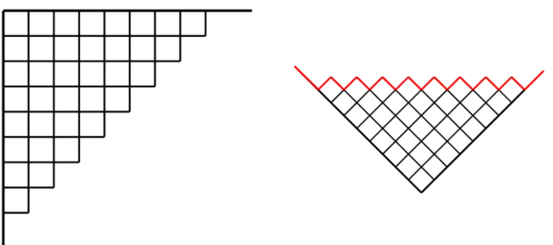
Figure 1: A Young diagram and the profile function(red line). left: A set of partitions(i.e. a Young diagram). right: A Russian style of the Young diagram and the profile function. The piecewise-linear function becomes the continuous function in the limitϵ1,2→ 0.
There are three different approaches to prove the correctness of the Nekrasov partition function[12, 28, 32, 33]. Since we discuss the Nekrasov and Okounkov approach for E-string theory in the next section, we review the approach only here. Their idea is to represent the sum of the partitions by that of the Young dia-grams(see the figure 1). The shape(the red line in the figure) is expressed by a piecewise-linear function fk(x) fk(x)= |x| + ∞ ∑ i=1 [ |x − ki+ i − 1| − |x − ki+ i| + |x + i| − |x + i − 1| ] . (2.14) We call this function the pro f ile f unction. In general, the profile function with
ϵ1,2is expressed as fk(x|ϵ1, ϵ2) = |x| + ∞ ∑ i=1 [ |x + ϵ1− ϵ2ki− ϵ1i| − |x − ϵ2ki− ϵ1i| − |x + ϵ1− ϵ1i| + |x − ϵ1i| ] , = |x| + ∞ ∑ j=1 [ |x + ϵ2− ϵ1˜kj− ϵ2j| − |x − ϵ1˜kj− ϵ2j| − |x + ϵ2− ϵ2j| + |x − ϵ2j| ] . (2.15)
This general profile function satisfies the following conditions
fk′(x|ϵ1, ϵ2) = ±1,
fk(x|ϵ1, ϵ2) ⩾ |x|, (2.16)
fk(x|ϵ1, ϵ2) = |x|, for |x| ≫ 0.
Moreover, the shifted profile function which is called a charged partition is defined by
fa;k(x|ϵ1, ϵ2)= fk(x− a|ϵ1, ϵ2). (2.17)
Then, the instanton charge a and the size of the partitions |k|, i.e. the size of the Young diagrams, are recovered from the charged profile function as
a = 1 2 ∫ R dx x fa;k′′ (x|ϵ1, ϵ2)= − 1 2 ∫ R dx fa;k′ (x|ϵ1, ϵ2), |k| = a2 2ϵ1ϵ2 − 1 4ϵ1ϵ2 ∫ dx x2fa;k′′ (x|ϵ1, ϵ2)= 1 2ϵ1ϵ2 ( a2− ∫ dx ( fa;k(x|ϵ1, ϵ2)− |x|) ) , (2.18) where the integral of the rightmost hand side of the first line is defined by the Caucy’s principal value one.
In the thermodynamic limitℏ → 0 or ϵ1,2→ 0, the typical size of the partition
k contributing to the partition function is given by|k| ∼ 1/ϵ1ϵ2. This means that
the size of a box in a Young diagram becomes small, namely the piecewise-linear profile function becomes a continuous profile function. Hence the sum of the par-titions can be approximated by an integral over the space of the continuous profile functions. This continuous profile function satisfies the following conditions7:
f (x) = |x|, |x| ≫ 0, | f (x) − f (y)| ⩽ |x − y|,∫ Rdx f ′(x) = 0, ∫ R dx( f (x)− |x|) < ∞, (2.19)
where the integral in the third condition is defined by the Caucy’s principal value one.
The approximation by the integral over the space of the continuous profile functions is the saddle point one. Namely, our task is to find the saddle point of the profile function from
Z⃗k(⃗a; ϵ1, ϵ2, Λ) = exp ( − 1 4 ∫ dxdy f′′ ⃗a,⃗k(x|ϵ1, ϵ2) f⃗a,⃗k′′ (y|ϵ1, ϵ2)γϵ1,ϵ2(x− y, Λ) ) , (2.20) where the integral is defined by the Caucy’s principal value one and γϵ1,ϵ2(x) is some function defined in Appendix A. Thus the partition function (2.11) becomes the sum over the profile functions
Z(⃗a; ϵ1, ϵ2, Λ) =
∑
f∈Γ⃗adiscrete
Zf(ϵ1, ϵ2, Λ), (2.21)
where Zf :=(2.20) and Γ⃗adiscreteis the set of the profile functions f = f⃗a,⃗k.
Viewing (2.20) as the action written with the profile function, the profile func-tion is known as the density f uncfunc-tion and the saddle point equafunc-tion obtained from the action is known as the loop equation in the matrix model8. Forϵ1, ϵ2 → 0,
(2.20) is expressed as Zf(⃗a; ϵ1, ϵ2, Λ) ∼ exp(EΛ ( f ) ϵ1ϵ2 ) , (2.22) where EΛ( f )= 1 4 ∫ y<x
dxdy f′′(x) f′′(y)(x− y)2(log( x − y
Λ ) − 3 2 ) , (2.23)
where the integral is defined as the Caucy’s principal value one. This is the leading term of the action (2.20) as ϵ1,2 → 0. The prepotential F0(⃗a, Λ) is given by the
saddle point of the action:
F0(⃗a, Λ) = −Critf∈Γ⃗a EΛ( f ), (2.24)
whereΓ⃗adenotes a set of the profile functions of the form
f (x) =
N
∑
l=1
fl(x− al), (2.25)
8For the good reviews of matrix model, see e.g. [36, 37], and as that closest to our discussion
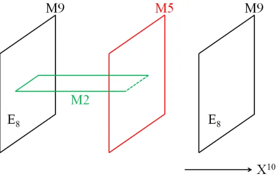
Figure 2: The formulation of E-string theory in terms of the M-theory picture. When the M5-brane approaches one of the M9-branes, the M2-brane becomes the non-critical, tensionless string.
with fl satisfying the conditions (2.19). This means, namely, that within all the
profile functions which dominate the Nekrasov partition function, only the critical points of the space of the profile functions, namely only the dominant profile functions give the prepotential.
For our main purpose, we will follow this idea in the later sections. There, we will recall this idea again and will discuss more concretely.
3
E-string Theory
In this section, we formulate E-string theory in terms of M-theory picture. We firstly see how E8symmetries appear and then how E-string theory is defined.
3.1
Formulation of E-string Theory
As said in Introduction, the history of E-string theory was started by P. Horava and E. Witten[4, 5]. They considered what type of M-theory can reproduce E8× E8
heterotic superstring theory in the limit where the M-theory direction becomes zero. Now we see the story briefly following the discussions of [4, 5](see the papers for more details).
First of all, we consider M-theory on an orbifoldR10×S1/Z2whereZ2acts on
S1as X10 → −X10and on the worldsheet as the orientation reversal. ThisZ
2action
breaks the original thirty-two supercharges to the half, i.e. sixteen supercharges. This means that if M-theory in the zero radius limit can reproduce one of the five known superstrings. It would be some one of Type I, E8×E8heterotic and S O(32)
heterotic superstrings.
Next, we consider the gravitational anomaly of M-theory on the orbifold. Then note that a metric onR10×S1/Z
2is same as one onR10×S1. We have a dynamical
metric on the orbifold, so we have its superpartner which has its spin 3/2 and is commonly called the Rarita-Schwinger field[17]. Though we would like to con-sider to obtain the effective action by integrating out the Rarita-Schwinger field, this eleven-dimensional Rarita Schwinger field has the gravitational anomaly be-cause it reduces in ten dimensions to a sum of infinitely many massive fields which are anomaly-free and the ten-dimensional Rarita-Schwinger field which is anoma-lous. Thus we have to know the form of the anomaly.
Under a spacetime diffeomorphism δXI = ϵvIwhere I runs over 0, 1, · · · , 10, ϵ is an infinitesimal quantity and vI a vector field, the change of the effective action
δΓ is generically written as δΓ = iϵ ∫ R10×S1/Z 2 d11X√gvI(X)WI(X), (3.1)
where g is the eleven-dimensional metric and WI(X) a function on the orbifold.
Thus that there does not exist the anomaly implies generically that WI(X) = 0.
However note that X is not on the orbifold points. Hence on the orbifold points, i.e. S1/Z
2 = [0, π], WI(X) is a sum of delta functions. We denote the orbifold
points on where the delta functions are defined, i.e. hyperplanes which are called the M9-branes later, by H′ and H′′respectively, following [4]. Then (3.1) can be decomposed into two parts
δΓ = iϵ ∫ H′ d10X√g′vIWI′+ iϵ ∫ H′′ d10X√g′′vIWI′′, (3.2)
where′ and ′′ means restrictions to H′ and H′′ respectively. This is the standard ten-dimensional anomaly. Therefore contributions of WI′ and WI′′ to the anomaly are even.
Here we have to care about that there are additional massless fields which live only on the hyperplanes. These are ten-dimensional vector multiplets. We have to count the number of these to cancel the anomaly. Though we have to recall the discussion of the Green-Schwarz mechanism[18] to proceed our discussion more precisely, we skip it and turn to the result directly.
To cancel the anomaly, we need 496 additional vector multiplets. This means that the superstring with sixteen supercharges has the gauge group whose dimen-sion is 496. As noted above, since contributions of the two hyperplanes to the anomaly is even, 496 is divided by two, which implies 248 each. This result shows that 248 vector multiplets, i.e. the gauge group whose dimension is 248, live on each hyperplane. E8× E8 heterotic superstring is only allowed in this
re-sult.
The picture which we have seen above was that the E8 gauge symmetry lives
on each end-of-the-world brane, i.e. the M9-brane. We now picture an addition of an M2-brane and an M5-brane between the M9-branes(see the figure 2).
We consider the M2-brane as oscillating modes on the M5-brane9. When the
M5-brane approaches one of the M9-branes(the left in the figure 2), the M2-brane looses one of three directions it spans and then it looks like a string. This string-like M2-brane is tensionless and non-critical[6, 20](and10 [21]). Such a string
is called the E-string. ”E ” of the name comes from the E8 symmetry as
fol-lows: firstly, E8 gauge fields live on the two M9-branes, but when the M5-brane
approaches one of the M9-branes, another M9-brane is much far from the M5-brane. Hence, it is too far for the world on the M5-brane where the E-string lives that it can be neglected and its E8 symmetry does not affect. Secondly, the E8
gauge symmetry on the M9-brane near by the M5-brane becomes the global
sym-9We can consider multiple M5-branes or M2-branes and in those cases, such theories are called
the E-string theories[19]. In this thesis, we are locked up in the usual E-string theory, i.e. one M2- and M5-brane.
10We have a comment on the references here. As mentioned in Introduction(footnote 2), before
considering the E8× E8 heterotic superstring theory with small instantons, the case of S O(32)
heterotic superstring was considered by Witten[7]. E8× E8and S O(32) heterotic superstrings are
not same but they are related with each other by T-duality, more precisely moduli spaces of them on S1are identical[22]. The string-like object was considered by Witten in type IIB superstring
on K3[21] and was called the non-critical string[20]. Based on these ideas, Ganor and Hanany studied the tensionless, non-critical string, namely E-string[6].
metry because it is out of the M5-brane. Hence, E-string theory has the E8global
symmetry and it is the origin of the name.
In addition, from the figure, it leaves only eight supercharges. By sending the parameterα′to zero whilst keeping the other physical parameters finite as done in the AdS/CFT correspondence[51], gravity is decoupled. Moreover, by taking the size of K3 to be large, the other modes except E-string are decoupled. Putting all together, E-string theory is the six-dimensional theory on the M5-brane with eight supercharges and the E8global symmetry.
Finally, we comment on fields in E-string theory. Actually, there is only one oscillating mode of the M2-brane. It is a tensor multiplet which decomposes into a vector multiplet when we perform dimensional reduction. In this sense, E-string theory is said to be the simplest theory as the six-dimensional(dynamical) the-ory. Nevertheless, we do not have its Lagrangian description yet, and in addition its least supersymmetry makes the control of E-string theory weak, so it is too difficult to analyse.
3.2
Two Prescriptions of E-string Theory
E-string theory is a (1,0) supersymmetric theory in six dimensions. The few su-percharges, i.e. eight susu-percharges, makes us lose control. To obtain theN = 2 theory in four dimensions by compactification, we must keep all the supercharges. This limitation leads us to toroidal compactificationR4× T2. However, this four-dimensional theory is basically asymptotically non-free11. Nevertheless, the
the-ory has the Seiberg-Witten description[10]. It is given by
y2 = 4x3− E4(τ) 12 u 4x− E6(τ) 216 u 6+ 4u5, ∂F0 ∂φ = 8π3i(φD− τφ) + const., (3.3)
where E4,6are the Eisenstein series,τ a modulus of the torus, φ, φDare the Higgs
vev and its dual, F0 the prepotential, and const. denotes terms which do not
de-pend on φ. We will recall this description again in the next section. Tracing the history ofN = 2 field theory, we naturally arrive at one more description, namely the Nekrasov partition function. However, we can hope but can hardly obtain
11It depends on the number of hypermultiplets. For simplicity, we will treat the theory as being
soon. Sakai hopefully searched and found it[13, 14]: Z = ∑ R ( e−2πiφ)|R| N ∏ k=1 ∏ (i, j)∈Rk ∏2N n=1ϑ1(21π(ak − mn+ ( j − i)ℏ), τ) ∏N l=1ϑ1(21π(akl+ hk,l(i, j)ℏ), τ)2 . (3.4) The details are given in the next section so we choose a short-cut. From this Nekrasov-type partition function, the prepotential is reproduced by
F0= (2ℏ2ln Z)|ℏ=0. (3.5)
Here we would like to focus on the higher order terms byℏ expansion. The virtue of the Nekrasov partition function (2.12) we have seen in the last section is to include the contribution of graviphotons in the higher order terms12. How about
in E-string theory? The answer is negative. The prepotential F0can be interpreted
as the genus zero topological string amplitude on local 12K3[34]. The all genus
amplitude is given by Z12K3 = exp (∑∞ g=0 ℏ2g−2F12K3 g ) . (3.6)
This amplitude satisfies the following holomorphic anomaly equation13[35]
∂E2Z 1 2K3= 1 24ℏ 2( 1 2πi∂φ )( 1 2πi∂φ+ 1 ) Z12K3. (3.7)
On the other hand, the Nekrasov-type partition function for E-string theory satis-fies the following modular anomaly equation
∂E2Z= 1 12ℏ 2( 1 2πi∂φ )2 Z (3.8) withℏ expansion Z = exp( 1 2ℏ2F0+ O(ℏ 0)). (3.9)
12In this papar, we did not treatϵ
1,2 expansion of the Nekrasov partition function. However,
in E-string theory, ℏ expansion corresponds to graviphoton expansion. For the details, see e.g. [38, 39, 34].
13We here call holomorphic anomaly equation, following the associated paper. However, since
the equation shows the dependence of the partition function on E2, we call it modular anomaly
For the genus zero topological string amplitude with massless hypermultiplets and the prepotential of E-string theory, (3.7) and (3.8) coincide with each other:
∂E2F0 = 1 24 ( 1 2πi∂φF0 )2 . (3.10) Thus we have F0 = F 1 2K3
0 |mi=0. However, for their higher order terms the anomaly
equations do not coincide. Hence we cannot say that the Nekrasov-type partition function for E-string theory include the contribution of graviphotons. Due to this reason, the discussions in the subsequent sections focus only on the genus zero part14.
4
Nekrasov-type Partition Function For E-string
The-ory
Thus far, we have reviewed some basics of E-string theory and analysis methods forN = 2 gauge theories in four dimensions. Historically, as we have seen in the last section, a major method for an analysis of E-string theory was the Seiberg-Witten description. We here give again the Seiberg-Seiberg-Witten description for E-string theory[10] y2 = 4x3− E4(τ) 12 u 4 x− E6(τ) 216 u 6+ 4u5, ∂F0 ∂φ = 8π3i(φD− τφ) + const., (4.1)
where E4,6are the Eisenstein series,τ a modulus of the torus, φ, φDare the Higgs
vev and its dual, and const. denotes terms which do not depend onφ.
In 2012, following the history, the Nekrasov-type partition function was appeared[13, 14] Z = ∑ R ( e−2πiφ)|R| N ∏ k=1 ∏ (i, j)∈Rk ∏2N n=1ϑ1(21π(ak− mn+ ( j − i)ℏ), τ) ∏N l=1ϑ1(21π(akl+ hk,l(i, j)ℏ), τ)2 , F0 = (2ℏ2ln Z)|ℏ=0, (4.2)
where R is a set of Young diagrams R = {R1, · · · , RN}, N comes from the U(N)
gauge theory15 . ϑ
1(z, τ) defined on the torus is one of the Jacobi theta functions
defined as(see appendix B for more details)
ϑ1(z, τ) := i ∑ n∈Z (−1)nyn−1/2q(n−1/2)2/2, ϑ2(z, τ) := ∑ n∈Z yn−1/2q(n−1/2)2/2, ϑ3(z, τ) := ∑ n∈Z ynqn2/2, ϑ4(z, τ) := ∑ n∈Z (−1)nynqn2/2. (4.3)
mn are fundamental matter masses and hk,l(i, j) are the relative hook lengths
de-fined between Young diagrams Rk and Rl. Most importantly,φ, τ and alare
abso-lutely different from (2.9). In (2.9), by q ∼ e2πiτ we had the UV coupling constant
τ but we now have the Higgs vev φ and τ is the modulus of the torus.
More-over, alin (2.9) were diagonal components of the Higgs vev but now they are just
constants on the torus. For consistency, we require a condition
2 N ∑ k=1 ak− 2N ∑ n=1 mn = 0. (4.4)
And concretely, for E-string theory we set
N = 4, ak = ωk−1 (k= 1 · · · , 4), mn = −mn+4 (n= 1, · · · , 4). (4.5)
This Nekrasov-type partition function was checked order by order and to satisfy some physical conditions. For instance, it satisfies the following modular anomaly equation ∂E2Z = ℏ2 12 1 (2πi)2∂ 2 E2Z. (4.6)
15This is a confusing problem. By the toroidal compactification, we have the N = 2 U(1)
gauge theory in four dimensions. However, the Nekrasov-type partition function can be viewed as the one generically for the U(N) gauge theory with 2N fundamental matters[13, 25]. We do not have the answer to the puzzle between them yet. Hence N does not have any physical meaning at present.
Substituting a relation between Nekrasov-type partition function and prepotential
Z = exp(1
2F0ℏ
−2+ O(ℏ0)) (4.7)
for this, we get
∂E2F0 = 1 24 ( 1 2πi∂φF0 )2 , (4.8)
which is the modular anomaly equation obtained from the Seiberg-Witten description[24]. However it did not have any proof for all orders in [13, 14]. In this section, we
give a proof[15] following [12].
4.1
Proof: Nekrasov and Okounkov approach
The basic idea of [12] is as follows. In the limitℏ → 0, which is called thermodynamic limit, we expect that there are some particular Young diagrams mainly contribut-ing the partition function. So we firstly have to specify the diagrams. This is done by the matrix model-like approach(see footnote 8). Next, under that situation, we can find an elliptic function. This gives the Seiberg-Witten description. The story flows in this order below.
For our purpose, it is convenient to rewrite the Nekrasov-type partition func-tion (4.2) as Z = ∑ R e2πi ˜φ|R|ZR, ZR = N ∏ k,l=1 ∞ ∏ i, j=1 (k,i),(l, j) ϑ1(21π(akl+ (µk,i− µl, j+ j − i)ℏ)) ϑ1(21π(akl+ ( j − i)ℏ)) × N ∏ k=1 2N ∏ n=1 ∏ (i, j)∈Rk ϑ1(21π(ak− mn+ ( j − i)ℏ)), (4.9) where ˜ φ := { φ if N is odd φ + 1 2 if N is even . (4.10)
Now we introduce a functionγ(z; ℏ) which satisfies a difference equation
γ(z + ℏ; ℏ) + γ(z − ℏ; ℏ) − 2γ(z; ℏ) = ln ϑ1
( z
2π
)
and which has the expansion(see appendix A for more details)
γ(z; ℏ) =∑∞
g=0
ℏ2g−2γ
g(z). (4.12)
Most importantly, we have the fact
γ′′ 0(z)= ln ϑ1 ( z 2π ) . (4.13)
Then, using this function, we can rewrite ZRas
ZR = exp [ − 1 4 ∫ dzdw f′′(z) f′′(w)γ(z − w; ℏ) + 1 2 2N ∑ n=1 ∫ dz f′′(z)γ(z − mn;ℏ) + N ∑ k,l=1 γ(ak− al;ℏ) − N ∑ k=1 2N ∑ n=1 γ(ak− mn;ℏ) ] , (4.14)
where the integrals are defined by the Cauchy’s principal value ones. The function
f (z) which is called a pro f ile f unction or its second derivative
f (z) = N ∑ k=1 [ℓ(Rk∑) i=1 (|z − ak− ℏ(µk,i− i + 1)| − |z − ak − ℏ(µk,i− i)|) +|z − ak+ ℏℓ(Rk)| ] , f′′(z) = 2 N ∑ k=1 [ℓ(Rk∑) i=1 (δ(z − a k− ℏ(µk,i− i + 1)) − δ(z − ak− ℏ(µk,i− i)) +δ(z − ak+ ℏℓ(Rk)) )] = 2 N ∑ k=1 [∑∞ i=1 (δ(z − a k − ℏ(µk,i− i + 1)) − δ(z − ak− ℏ(µk,i− i)) −δ(z − ak+ ℏ(i − 1)) + δ(z − ak − ℏi))+ δ(z − ak) ] (4.15)
knows Young diagrams mainly contributing to the partition function (4.14) since the delta functions within the profile function characterise the shapes of them[12]. Such a function f′′(z) can be viewed as a density function in matrix model. We
assume that they are separated from each other. Let z = ak be points where the
delta functions take values,Ckbe the local support around them, andC their union
C =∪N
k=1Ck. Then it follows that
ak = 1 2 ∫ Ckz f ′′(z)dz, |R| = 1 4 ∫ Cdzz 2 f′′(z)− N ∑ k=1 a2k 2. (4.16)
Then the original partition function (4.9) can be approximated by an integral over the space of the delta functions
Z ≃ ∫ D f′′dNλ exp( 1 2ℏ2F0+ O(ℏ 0)), (4.17) where F0[ f′′, λk] = − 1 2 ∫ C dzdw f′′(z) f′′(w)γ0(z− w) + 2N ∑ n=1 ∫ C dz f′′(z)γ0(z− mn) +4πi ˜φ(1 4 ∫ Cdzz 2 f′′(z)− N ∑ k=1 a2 k 2 ) +2 N ∑ k=1 λk (1 2 ∫ Ck dzz f′′(z)− ak ) , (4.18)
where the integrals of the first line are defined by the Cauchy’s principal value ones and we have introduced Lagrange multipliersλk taking account of the constraints
(4.16). Here we have to care about the function F0, which is slightly different
from the prepotential F0as we will see later.
In this situation, we take the thermodynamic limit ℏ → 0. Then, there are some dominant Young diagrams in (4.17) and the delta functions know them. We evaluate the partition function (4.17) by the saddle point approximation. We obtain, by the variation ofF0with respect to f′′(z)
∫ C dw f′′(w)γ0(z− w) − 2N ∑ n=1 γ0(z− mn)− πi ˜φz2− λkz= 0, z ∈ Ck. (4.19)
This saddle point equation can be viewed as the loop equation in matrix model. We would like to solve this equation but it is generically a big problem. Here we
introduce an analytic function Ω(z) := ∫ C f′′(w)γ′′0(z− w)dw − 2N ∑ n=1 γ′′ 0(z− mn) = ∫ C f ′′(w) lnϑ 1 (z − w 2π ) dw− 2N ∑ n=1 lnϑ1 (z − mn 2π ) . (4.20) We use this function instead of f′′ to solve the saddle point equation. Moreover, recalling matrix model, we define the resolventω(z) using the function above as
ω(z) := Ω′(z). (4.21)
By this definition, we called the functionΩ(z) the antiderivative o f the resolvent in the paper[15]. Then the function f′′ is recovered as
2πi f′′(z)= ω(z − iϵ) − ω(z + iϵ), z ∈ C, (4.22)
whereϵ = δz is an infinitesimal deformation along the cuts.
We consider the second derivative of the saddle point equation (4.19) with respect to z:
1
2(Ω(z − iϵ) + Ω(z + iϵ)) − 2πi ˜φ = 0, z ∈ C. (4.23)
We now solve this. To do it, we introduce a meromorphic function on the torus, whose poles are at z = mn
G(z) := eΩ(z)−2πi ˜φ+ e−Ω(z)+2πi ˜φ, (4.24) whilst the function Ω(z) has logarithmic branch points as well as square root branch points. By the condition (4.4), G(z) is doubly periodic, i.e. it is an el-liptic function of order 2N on the torus. Using this function, the resolvent can be written as
ω(z) = √ G′(z)
(G(z)+ 2)(G(z)) − 2. (4.25) Let us count the number of the branch points. Since G(z)± 2 have 2N branch points each, ω(z) has totally 4N branch points. However, the actual ω(z) should have 2N branch points. This mismatch is resolved if the function
H(z) := G(z)+ 2 4 = cosh 2(1 2(Ω(z) − 2πi ˜φ) ) (4.26)
has N zeroes of multiplicity two instead of 2N simple zeroes. The singularities of
H(z) are the single poles at z= mn. Such an elliptic function is determined as
H(z)= κP(z) 2 Q(z) = κ (∏Nk=1ϑ1( z−ζk 2π )) 2 ∏2N n=1ϑ1(z−mn2π ) , (4.27)
where κ and ζk are some constants. The locations of zeroes and poles have to
satisfy 2 N ∑ k=1 ζk − 2N ∑ n=1 mn= 0. (4.28)
Here the equality should be understood modulo periods of the torus. Then the antiderivativeΩ(z) is obtained as
Ω(z) = 2 ln( √H(z)+ √H(z)− 1)+ 2πi ˜φ, (4.29)
and therefore, the resolvent is obtained as
ω(z) = 2∂z
√ H(z) √
H(z)− 1. (4.30)
Finally, we make a comment on the constantζk. The function f′′has to satisfy
the constraint (4.16). In terms of the resolvent, it is expressed as
ak =
1 4πi
I
γkzω(z)dz. (4.31)
This holds ifω(z) satisfies
ω(ak− z ± iϵ) = ω(ak + z ± iϵ) for ak+ z ∈ Ck. (4.32)
This holds if the function H(z) satisfies
√
H(ak − z) = −
√
H(ak+ z) for ak+ z ∈ Ck. (4.33)
4.2
The case of E-string theory
We here focus on the case of E-string theory, i.e. with the E8global symmetry. In
this case, the setup is given by
N = 4, ζk = (0, π, −π − πτ, πτ), mn = (0, 0, 0, 0) (4.34)
or[13]
N = 3, ζk = ωk = (π, −π − πτ, πτ), mn = (0, 0, 0). (4.35)
We here choose the latter. Then the functions P(z) and Q(z) are expressed as
P(z)= −iq−1/4 3 ∏ k=1 ϑk+1 ( z 2π ) , Q(z) = ϑ1 ( z 2π )6 . (4.36)
Therefore the function H(z) is written as
H(z)= −1
4u℘
′(z)2, (4.37)
where we have used the identity
℘′(z)2 = η12 3 ∏ k=1 ϑk+1(2zπ)2 ϑ1(2zπ)2 . (4.38)
Here℘′(z) is the derivative of the Weierstrass’ elliptic function and η := η(τ) the Jacobi eta function. Also, we have defined the parameter u as
u := 4κ
q1/2η12. (4.39)
Then the resolvent is written as
ω(z) = √ 2℘′′(z)
℘′(z)2+ 4u−1. (4.40)
This Riemann surface has three cuts near z = ωk and the three cuts shrinks as
|u| increases. In particular, when u is sent to infinity, all cuts disappear and the
Riemann surface becomes the torus. This is reminiscent of the classical limit of the Seiberg-Witten curve (4.1) and therefore lets us identify u with the Coulomb branch moduli parameter.
Next we would like to consider the Seiberg-Witten description, i.e. theα- and
β-cycle integrals. We first consider the α-cycle integral. To do this, we use the
following fact 1 2π2i I α lnϑ1(z − w 2π ) dz= C1(τ) mod Z, (4.41)
where C1(τ) is some function in τ. An important thing is not the explicit form
of C1(τ) but that C1(τ) is independent of w and invariant under continuous
defor-mation of the integration contour. This fact can be shown as follows: since the theta function is quasi-periodic ϑ1(z+ 1) = −ϑ1(z), the function 21πilnϑ1(z2−wπ )2 is
single-valued modulo Z along a loop belonging to the cycle α. Recall also that the theta function is regular for|z| < ∞, so that the integral is invariant under the continuous deformation of the loop.
Now we use the fact (4.41) with the function (4.20). And also we know f′′ to be a set of the delta functions from (4.15). Hence we obtain
1 2π2i I αΩ(z)dz = 1 2π2i I α ∫ C f′′(w) lnϑ1(z − w 2π ) dwdz − 1 2π2i I α 2N ∑ n=1 lnϑ1(z − m n 2π ) dz modZ, =⇒ 1 4π2i I αΩ(z)dz = 0 mod Z, (4.42)
where C1’s cancel with each other. Here using the relation betweenΩ(z) and H(z),
(4.29), we obtain ˜ φ = i 2π2 I α ln( √H(z)+ √H(z)− 1)dz modZ. (4.43)
Now we have arrived at the important stage where we give the Seiberg-Witten description explicitly. Recalling that the function H(z) includes the Coulomb moduli parameter u, we differentiate the Higgs vev (4.43) with respect to u:
∂φ ∂u = i 4π2u I α dz √ 1− H(z)−1. (4.44)
Note that this is not affected by the difference between φ and ˜φ = φ + 12. In the case of the E-string theory with the E8 global symmetry, the function H(z) was
given by (4.37). Therefore we get ∂φ ∂u = i 4π2u I α ℘′(z)dz √ ℘′(z)2+ 4u−1. (4.45)
The Seiberg-Witten curve should be given as the Riemann surface of the integrand. However, we have to pay attention to that the double-periodic sheet has three cuts near z = ωk and we have two copies of it. Hence, whilst the Seiberg-Witten curve
is of genus one, the Riemann surface of the integrand is of genus four. To solve this problem, we use the identity
℘′(z)2 = 4℘(z)3− E4(τ)
12 ℘(z) −
E6(τ)
216 (4.46)
and perform a change of variables as
℘(z) = u−2x. (4.47) Then (4.45) is expressed as ∂φ ∂u = i 4π2 I ˜ α dx y , (4.48)
where ˜α is the image of α by the map (4.47) and y is given by
y2 = 4x3− E4(τ) 12 u 4 x− E6(τ) 216 u 6+ 4u5. (4.49)
This is exactly the Seiberg-Witten curve for the E-string theory (4.1). Thus one of the Seiberg-Witten description has been reproduced from the Nekrasov-type partition function.
Next we would like to reproduce the relation between the prepotential and the Higgs vev, i.e. consider the beta-cycle integral. To do this, we need two ingredients: the modular transformation law of the theta function
ϑ1 ( z 2π, τ ) = e3πi/4τ−1/2exp(− iz2 4πτ ) ϑ1 ( z 2πτ, − 1 τ ) (4.50)
and the fact (4.41) with the modulus−1/τ. Then we can show that 1 2π2iτ ∫ z0+2πτ z0 lnϑ1 (z − w 2π , τ ) dz = − 1 8π3τ2 ∫ z0+2πτ z0 (z− w)2dz + 1 2π2iτ ∫ z0+2πτ z0 lnϑ1(z − w 2πτ , − 1 τ ) dz+ 3 4− 1 2πilnτ = − 1 8π3τ2 ∫ z0+2πτ z0 (z− w)2dz+ C1 ( − 1 τ ) + 3 4 − 1 2πilnτ mod Z = − 1 4π2τw 2+( 1 2π + z0 2π2τ ) w+ C2(z0, τ) mod Z, (4.51)
where C2(z0, τ) is some function in z0 and τ. Putting this, (4.15) and (4.20)
to-gether, we obtain 1 4π2iτ ∫ z0+2πτ z0 Ω(z)dz = − 1 8π2τ ∫ C w2f′′(w)dw+( 1 4π + z0 4π2τ ) ∫ C w f′′(w)dw modZ = i 8π3τ (∂F0 ∂φ + 2πi N ∑ k=1 a2k)+( 1 2π + z0 2π2τ )∑N k=1 ak modZ. (4.52)
C2’s cancel with each other in the first equality and the integrals with respect to w
are defined by the Caucy’s principal value ones. To show the second equality, we have used (4.16) and (4.18) with
∂F0 ∂φ = ∂F0 ∂φ extremum = [(∂F0 ∂φ ) f′′ + (δF0 δ f′′ ) φ ∂ f′′ ∂φ ] extremum =[(∂F0 ∂φ ) f′′ ] extremum . (4.53) Here (∂F0/∂φ)f′′ denotes the partial derivative ofF0with respect toφ, holding f′′
constant.
Now we focus on the E-string theory with the E8global symmetry. Since the
setup
the integral (4.52) becomes 1 4π2iτ ∫ z0+2πτ z0 Ω(z)dz = i 8π3τ (∂F0 ∂φ + 2πi 3 ∑ k=1 ω2 k ) . (4.55)
Hence the integral does not depend on the choice of z0 and this result makes the
integral the beta-cycle one, i.e. 1 4π2iτ I βΩ(z)dz = i 8π3τ (∂F0 ∂φ + 2πi 3 ∑ k=1 ω2 k ) . (4.56)
Now we have arrived at the point where we can obtain the Seiberg-Witten descrip-tion. Firstly, using (4.29), the l.h.s. of (4.56) is written as
1 4π2iτ I βΩ(z)dz = 1 2π2iτ I β ln( √H(z)+ √H(z)− 1)dz+ ˜φ = −1τφD+ φ + const., (4.57)
where we have identified the dual Higgs vevφDas
φD = i 2π2 I β ln( √H(z)+ √H(z)− 1)dz+ const. (4.58)
from the analogy of (4.43). Here const.’s are some functions inτ but are indepen-dent ofφ. Secondly, the summation term of the r.h.s. of (4.56) can be written as const. becauseωkconsists ofπ and τ only. Puttinig all together, hence, we finally
obtain
∂F0
∂φ = 8π3i(φD− τφ) + const.. (4.59)
5
The Generalisation to the Cases with Wilson Lines
In the previous section, we proved that the Nekrasov-type partition function for E-string theory is correct, namely starting the Nekrasov-type partition function we can reproduce the Seiberg-Witten description. E-string theory we have seen is the simplest case in the sense that the theory does not have any Wilson lines. Therefore the natural question arises: is the Nekrasov-type partition function also correct in the cases with Wilson lines? In this section, we answer the questionpositively in a sense that the Nekrasov-type partition function with Wilson lines
can reproduces the Seiberg-Witten curve. However, as mentioned in section 3, the higher order terms in theℏ expansion cannot interpret the graviphoton expansion as in the original Nekrasov partition function. Hence we stress again that we focus on the genus zero part. We discuss the cases with three Wilson lines firstly and the cases with four Wilson lines secondly. And also, we focus only on the alpha-cycle integral (4.44).
5.1
The cases with three Wilson lines
In these cases, we choose16
N = 3, ζk = ωk, mn = (2πm1, 2πm2, 2πm3). (5.1)
Then the function H(z) is written as
H(z) = κ( ∏3 k=1ϑ1( z−ζk 2π )) 2 ∏6 n=1ϑ1(z−2πmn2π ) = κ ϑ1( z−π 2π) 2ϑ 1(z+π+πτ2π )2ϑ1(z−πτ2π )2 ϑ1(z−2πm2π 1)2ϑ1(z−2πm2π 2)2ϑ1(z−2πm2π 3)2ϑ1(z+2πm2π 1)2ϑ1(z+2πm2π 2)2ϑ1(z+2πm2π 3)2 . (5.2) We need two tools here. One, we need the transformation laws of the theta func-tions which are given in Appendix B for the numerator. And two, we need the identity ϑ1 (z + w 2π ) ϑ1 (z − w 2π ) = −η−6ϑ 1 ( z 2π )2 ϑ1 ( w 2π )2 (℘(z) − ℘(w)) (5.3)
16In this section, we take the Wilson lines to be not m
for the denominator. Then we can express the function (5.2) written in terms of the theta functions which depend on z as the Weierstrass℘-functions and obtain
H(z) = κη 6℘′(z)2 q1/2ϑ 1(m1)2ϑ1(m2)2ϑ1(m3)2(℘(z) − ℘(2πm1))(℘(z) − ℘(2πm2))(℘(z) − ℘(2πm3)) = uη18℘′(z)2 4ϑ1(m1)2ϑ1(m2)2ϑ1(m3)2(℘(z) − ℘(2πm1))(℘(z) − ℘(2πm2))(℘(z) − ℘(2πm3)) , (5.4) where we have used the moduli parameter (4.39). To proceed the story following
the last section, we would like to identify the Seiberg-Witten curve in the alpha-cycle integral (4.44) in the present case. The integrand of the alpha-alpha-cycle integral (4.44) is now written as dz √ 1− H(z)−1 = √ H(z)dz √ H(z)− 1 = ℘′(z)dz √ ℘′(z)2− α(m)(℘ − ℘ 1)(℘ − ℘2)(℘ − ℘3) , (5.5) where α(m) := 4 uη18ϑ1(m1) 2ϑ 1(m2)2ϑ1(m3)2, ℘i := ℘(2πmi). (5.6)
By a change of variables ℘(z) = x, we identify this integrand written in terms of the variable x with the Seiberg-Witten curve, i.e. we put
y20 = ℘′(z)2− α(m)(℘(z) − ℘1)(℘(z) − ℘2)(℘(z) − ℘3)
= (4 − α)℘3+ ασ
1℘2− (E4+ ασ2)℘ − (E6− ασ3), (5.7)
where
σ1 := ℘1+ ℘2+ ℘3, σ2 := ℘1℘2+ ℘2℘3+ ℘1℘3, σ3 := ℘1℘2℘3, (5.8)
and we have dropped the coefficients of E4 and E6, namely we defined E′4 :=
E4/12 and E′6 := E6/216 and then we dropped the prime. For later convenience,
we change the variable z into x below. We have to now recall that the sheet which the functions are defined has three cuts and we have two copies of them. Hence the curve (5.7) is of genus four. To obtain the genus one curve, taking into account that the curve (5.7) is inCP2, we perform the appropriate change of variables as
More concretely and explicitly, we follow the computation minutely and so we take five steps to make the curve (5.7) be the correct Seiberg-Witten curve: one is to redefine the variables, two to eliminate the second-order term, three to redefine the variables, four to didvide byα6and redefine the variables to rewriteα into the
modulus u, and five to express the curve in terms of the modulus u. First step, we multiply both sides of (5.7) by (4 − α)2 and perform a change of variables
x0 := (4 − α)℘:
(4− α)2y20 = x30+ ασ1x20− (E4+ ασ2)(4− α)x0− (4 − α)2(E6− ασ3). (5.10)
Second step, we perform a shift x0 = x − ασ1/3 to eliminate the square term of
x0: (4− α)2y20 =(x− ασ1 3 )3 + ασ1 ( x− ασ1 3 )2 −(E4+ ασ2)(4− α) ( x− ασ1 3 ) − (4 − α)2 (E6− ασ3). (5.11) From this, we get the curve
(4− α)2y20 = x3− ˜fx − ˜g. (5.12)
Third step, multiplying both sides of (5.12) by four and redefining the variable y0
as y := 2(4 − α)y0, we get the curve
y2= 4x3− f x − g, (5.13) where f := 4 ˜f and g := 4˜g: f = 16E4+ (16σ2− 4E4)α + (4σ2 1 3 − 4σ2 ) α2, g = 64E6− (16 3 E4σ1+ 32E6+ 64σ3 ) α + (4E6+ 4 3E4σ1− 16 3 σ1σ2+ 32σ3 ) α2−( 8 27σ 3 1− 4 3σ1σ2+ 4σ3 ) α3. (5.14) Fourth step, dividing both side of (5.13) byα6, the curve (5.13) becomes
y2 α6 = 4 x3 α6 − f α4 x α2 − g α6. (5.15)
We redefine the variables as
˜y := y/α3, ˜x := x/α2. (5.16)
Then the curve (5.15) is written as
˜y= 4 ˜x3− f′˜x− g′, (5.17) where f′ := f /α4and g′:= g/α6: f′ = 16E4α−4+ (16σ2− 4E4)α−3+ (4σ2 1 3 − 4σ2 ) α−2, g′ = 64E6α−6− (16 3 E4σ1+ 32E6+ 64σ3 ) α−5 + (4E6+ 4 3E4σ1− 16 3 σ1σ2+ 32σ3 ) α−4−( 8 27σ 3 1− 4 3σ1σ2+ 4σ3 ) α−3. (5.18) Thus far, we have taken four steps to get the correct Seiberg-Witten curve, i.e. we wanted the genus one curve, the Weierstrass form, and the expression in terms of the modulus u as the ingredients. To rewrite α into the modulus u is the rest of the steps. Fifth step, finally, we do it. However, that we have stopped here is not that we waste the time because by this step an important result is shown. Now we recallα(m) := 4ϑ1(m1)2ϑ1(m2)2ϑ1(m3)2/uη18. So we define the new modulus ˜u as
˜u := α−1= η
18
ϑ1(m1)2ϑ1(m2)2ϑ1(m3)2
u. (5.19)
Then (5.18) is rewritten as
f′ = 16E4˜u4+ (16σ2− 4E4) ˜u3+
(4σ2 1 3 − 4σ2 ) ˜u2, g′ = 64E6˜u6− (16 3 E4σ1+ 32E6+ 64σ3 ) ˜u5 + (4E6+ 4 3E4σ1− 16 3 σ1σ2+ 32σ3 ) ˜u4−( 8 27σ 3 1− 4 3σ1σ2+ 4σ3 ) ˜u3. (5.20) This curve is the Seiberg-Witten curve we wanted. We can check the correctness by comparing this curve with the curve obtained in [26], i.e. this curve is in
agreement with the curve obtained in [26]17. However, the author guess that the
judicious reader notices that this curve (5.20) is divergent at mn = 0. To solve the
problem, we take one step further. We recall the new modulus (5.19). The curve is written in terms of the new modulus. The one step we need is to take the new modulus ˜u back to the old modulus u. Namely, we rewrite the curve (5.20) as
f′ = 16E4 ( η18 ϑ1(m1)2ϑ1(m2)2ϑ1(m3)2 u)4+ (16σ2− 4E4) ( η18 ϑ1(m1)2ϑ1(m2)2ϑ1(m3)2 u)3 + (4σ21 3 − 4σ2 )( η18 ϑ1(m1)2ϑ1(m2)2ϑ1(m3)2 u)2, g′ = 64E6 ( η18 ϑ1(m1)2ϑ1(m2)2ϑ1(m3)2 u)6−(16 3 E4σ1+ 32E6+ 64σ3 )( η18 ϑ1(m1)2ϑ1(m2)2ϑ1(m3)2 u)5 + (4E6+ 4 3E4σ1− 16 3 σ1σ2+ 32σ3 )( η18 ϑ1(m1)2ϑ1(m2)2ϑ1(m3)2 u)4 − ( 8 27σ 3 1− 4 3σ1σ2+ 4σ3 )( η18 ϑ1(m1)2ϑ1(m2)2ϑ1(m3)2 u)3. (5.22)
Then multiplying the whole of the curve with these coefficients by (4ϑ1(m1)2ϑ1(m2)2ϑ1(m3)2/η18)6,
we obtain (4ϑ1(m1)2ϑ1(m2)2ϑ1(m3)2 η18 )6 ˜y2 = 4(4ϑ1(m1) 2ϑ 1(m2)2ϑ1(m3)2 η18 )6 ˜x2 − (4ϑ1(m1)2ϑ1(m2)2ϑ1(m3)2 η18 )6 f′˜x − (4ϑ1(m1)2ϑ1(m2)2ϑ1(m3)2 η18 )6 g′. (5.23)
17For the perfect match up to the numerical factors, note that the difference between the
nota-tions is
16E4ours= f0Mohri′s, 64Eours6 = g0Mohri′s, 4℘oursi = ℘Mohrii ′s. (5.21) In addition, we have two more terms−32E6˜u5and 32σ3˜u4and a different coefficient of −64σ3˜u5
compared with the Mohri’s result (9.18) in [26]. But we checked that those two terms and the coefficient of (9.18) have been stolen.
Finally, we redefine the variables and the coefficients as Y := (4ϑ1(m1) 2ϑ 1(m2)2ϑ1(m3)2 η18 )3 ˜y, X := (4ϑ1(m1) 2ϑ 1(m2)2ϑ1(m3)2 η18 )2 ˜x, F := (4ϑ1(m1) 2ϑ 1(m2)2ϑ1(m3)2 η18 )4 f′, G := (4ϑ1(m1) 2ϑ 1(m2)2ϑ1(m3)2 η18 )6 g′. (5.24) Then we obtain Y2 = 4X3− FX − G, F = 16E4u4+ (16σ2− 4E4)α′(m)u3+ (4σ2 1 3 − 4σ2 ) α′(m)2u2, G = 64E6u6− (16 3 E4σ1+ 32E6+ 64σ3 ) α′(m)u5 + (4E6+ 4 3E4σ1− 16 3 σ1σ2+ 32σ3 ) α′(m)2u4−( 8 27σ 3 1− 4 3σ1σ2+ 4σ3 ) α′(m)3u3, α′(m) := 4ϑ1(m1)2ϑ1(m2)2ϑ1(m3)2 η18 , (i.e. α(m) = α ′(m)/u). (5.25)
We can easily see that this curve is not divergent at mn= 0 and gives the
Seiberg-Witten curve for the E-string theory with the E8 global symmetry. We can take
the limit limm→0℘(2πm)ϑ1(m)2 = η6. By using this in (5.25), we obtain
Y2= 4X3− 16E4u4X− 64E6u6+ 256u5, (5.26)
where the last term 256u5 comes from the term −64σ
3α′(m)u5 within G. This
is precisely the Seiberg-Witten curve for the E-string theory with the E8 global
symmetry18.
By the discussion we have seen thus far, it was shown that the Nekrasov-type partition function gives the Seiberg-Witten curves also in the cases with three Wilson lines. And also, it was shown that, comparing our result with the result obtained in [26], ours explicitly includes the dependence of the Seiberg-Witten curve on the Wilson lines.
18For the reader who does not like the different numerical factors, the redefinition X
new:= Xold/4
5.2
The cases with four Wilson lines
In these cases, we choose the setup as
N = 4, ζk = (0, ωi), mn= (2πm1, 2πm2, 2πm3, 2πm4). (5.27)
This is the most general setup. The function H(z) is given by
H(z) = κ( ∏4 k=1ϑ1(z−ζk2π ))2 ∏8 n=1ϑ1(z−mn2π ) = κ ϑ1( z 2π) 2ϑ 1(z2−ππ)2ϑ1(z+π+πτ2π )2ϑ1(z−πτ2π )2 ϑ1(z−2πm2π 1)· · · ϑ1(z−2πm2π 4)ϑ1(z+2πm2π 1)· · · ϑ1(z+2πm2π 4) . (5.28) Following the discussion in the previous subsection, we obtain
y20 = ℘′(z)2+ α(m)(℘(z) − ℘1)(℘(z) − ℘2)(℘(z) − ℘3)(℘(z) − ℘4) = 4℘3− E 4℘ − E6+ α(℘4− σ1℘3+ σ2℘2− σ3℘ + σ4), (5.29) where α(m) := 4 uη24ϑ1(m1) 2ϑ 1(m2)2ϑ1(m3)2ϑ1(m4)2, σ1 := ℘1+ ℘2+ ℘3+ ℘4, σ2 := ℘1℘2+ ℘2℘3+ ℘3℘4+ ℘1℘3+ ℘1℘4+ ℘2℘4, σ3 := ℘1℘2℘3+ ℘1℘2℘4+ ℘1℘3℘4+ ℘2℘3℘4, σ4 := ℘1℘2℘3℘4. (5.30)
This curve (5.29) is superficially a quartic curve. To get a cubic curve, we need two tools. Firstly, we restore the homogeneous coordinates as19
x1 = ℘, x2 = y0, , x0 , 1. (5.31)
Secondly, we recall the fact that the curve (5.29) is
x0x22 = 4x 3
1− E4x20x1− E6x30 (5.32)
19In the cases with three Wilson lines we saw in the previous subsection, one of the