西 南 交 通 大 学 学 报
第 55 卷 第 1 期
2020 年 2 月
JOURNAL OF SOUTHWEST JIAOTONG UNIVERSITY
Vol. 55 No. 1
Feb. 2020
ISSN: 0258-2724 DOI:10.35741/issn.0258-2724.55.1.7
Research Article Mathematics
R
EFUGE AND
A
GE
S
TRUCTURES
I
MPACT ON THE
B
IFURCATION
A
NALYSIS OF AN
E
COLOGICAL
M
ODEL
改造和年龄结构对生态模型分叉分析的影响
Azhar1Abbas Majeed
Departmentof Mathematics, Collegeof Science, University of Baghdad Al-Jadriya, Karrada, 10071, Baghdad, Iraq
[email protected] Abstract
In this paper, the conditions of the incidence of the local bifurcation, such as a saddle-node pitchfork bifurcation and transcritical of an ecological system (consistingprey shelter (refuge) and age stages for both populations) considered to study. Lotka-Volterra type of functional response was suggested. Subsequently, the inquiry and analysis are remarked that the transcritical bifurcation transpires close to the equilibrium (symmetry) point , in addition to the incidence of asaddle-node bifurcation at symmetry points and . It should be mentioned that there is no likelihood of the incidence of the pitchfork bifurcation at every single point. In conclusion,s to illustrate the incidence of the local bifurcation of this system, some simulations were used. The aim of this study is to examine the effect of each parameter on the stability of equilibrium points.
Keywords: Prey-Predator, Refuge, Stage-Structure, Local Bifurcation, Sotomayor's Theorem
摘要 本文研究了局部分支发生的条件,例如马鞍节点的干草叉分支和生态系统的跨临界(由两个种 群组成的避难所(避难所)和年龄阶段)进行研究。建议使用洛特卡 - 沃尔泰拉类型的功能性反应。 随后,进行询问和分析时,除了在对称点和上出现鞍形节点分叉以外,跨临界分叉点还靠近平衡点( 对称点)。应该提到的是,在每个点上都不会出现干草叉分叉的可能性。总之,为了说明该系统局部 分叉的发生率,使用了一些模拟。这项研究的目的是检查每个参数对平衡点稳定性的影响。 关键词: 捕食者,避难所,阶段结构,局部分支,索托马约尔定理
I. I
NTRODUCTIONThe predator-prey model is a very important tool in ecology in order to understand the interaction between populations in the natural environment. Factors that affect the population are assessed by one of the study disciplines of ecology, namely the biology of the population. A
population is defined as a group of identical species residing in a similar geographical area. In recent times, researchers have focused on the general factors of population components to assess these populations. When a population biologist wants to evaluate a species, it uses severaltools to obtain information. Mathematical formulas and
paradigms are assembled based on the experimentations and remarks and then depleted to make prognostications. Fundamentally, the scholars ought to look at aspects that influence the populace [1].
A strategy that protects prey from predation and reduces the risk of predation is the use of shelters (refuges), where they play an important role and have a significant impact on the co-existence of predator and prey. In the literature, there are two types of refuges: the first that protects a constant number of prey and the second that protects a constant proportion of prey [2], [3].
Abdulghafour and Naji [4] studied a mathematical model of a prey-predator system with infectious disease in the prey population. It is assumed that there is a constant refuge in prey, as a defensive property against predation and harvesting from the predator.
Age factor is just as important as shelter for living organisms,whichreproduction and growth rate depends on age. Also, it was observed that the life history of many species goes through at least two phases, i.e., immature and mature. In the first stage, species cannot interact with others and reproduction, as they depend on their parentsfor food and breeding. In the last three decades, several prey-predator models with stage-structure have been proposed and analysed [5], [6], [13].
Beay et al. [7] suggested and examined the local steadiness of the Rosenzweig-MacArthur predator-prey scheme with Holling type-II operative rejoinder, and stage-structure is examined for prey in this research.
The name "bifurcation" was first introduced by Henri Poincaré in 1885 in his first mathematics paper, showing such behavior. Moreover, the bifurcation occurs in both continuous (described by ordinary differential equations) [8], [9] and discrete systems’ (illustrated by maps) [10], [11]. The bifurcation is split up into two fundamental classes: local bifurcations and global bifurcations. Local bifurcations can be examined entirely via alters in the local steadiness properties of equilibrium periodic orbit, while global bifurcations occur when larger periodic orbits collide with equilibrium. This triggers variations in the topology of the tracks in stage space, which cannot be narrowed to a trifling vicinity, as is the instance with indigenous.
Bifurcations Pamuk and Cay in [12] studied the steadiness and Hopf bifurcation analysis of a feedback diffusion technique, which shapes the communication among endothelial cells and inhibitors.
In this paper, the conditions of the incidence of the indigenous bifurcationare considered to review, such as saddle-node transcritical and pitchfork for a mathematical paradigm comprising of stage-structured inprey, in addition to predator andprey refuge. Lotka-Volterra form of functional rejoinder was suggested after the examination and analysis.
It is noticed that the transcritical bifurcation occurs near the equilibrium (symmetry) point , in addition to the incidence of the saddle-node bifurcation at equilibrium (symmetry) points and . It is valuable to state that there is no likelihood incidence of the pitchfork bifurcation at every single step. Conclusively, certain numerical imitations are expended to illustrate the incidence of the local bifurcation of this paradigm.
A. The Mathematical Paradigm
Consider the following ecological model:
,
with initial conditions:
(0) and W (0)
where the parameters of this model are illustrated in Table 1:
Table 1.
The parameters of System (1)
X(t) Immature prey populace at time t Y(t) Mature prey populace at time t Z(t) Immature predator populace at time t W(t) Mature predator populace at time t
Inherent growth level of immature prey The carrying capacity The grown-up rate of immature prey
individuals onto mature prey The natural death rate of immature prey The natural death rate of immature prey
prey species from predation by the predator
The grown-up rate of immature predator individuals onto mature
predators
The predation rate of mature prey by a predator
The conversion rate of food The natural death rate of an immature
predator in the absence of prey The natural death rate of a mature
predator in the absence of prey
Not that the directly above suggested that the paradigm has 12 parameters, all of which make the enquiry problematic. Thus, as to make things easier for the scheme, the number of parameters wasabridged by means of the subsequent dimensionless variables and parameters:
Next, the non-dimensional kind of the Scheme (1) can be described as:
where
and
It is remarked that the quantity of parameters hasbeen abridged from 12 in the Scheme to (8); in the Scheme [2].
B. The Equilibrium Points of System (2)
Scheme has a maximum number of three equilibrium (symmetry) points,which aredetailed in the subsequent paragraph:
The equilibrium (symmetry) point the free predator equilibrium point and the positive
(coexistence) equilibrium point ).
C. Local Bifurcation Analysis
In this sector, conditions are examined for bifurcation. Thus, in the following theorems and applications, Sotomayor's theorem is appropriate for the local bifurcation.
Now, the Jacobian matrix of Scheme is:
To substantiate, it is obvious that for any nonzero vector ; we have:
where and is any
bifurcation parameter. In the subsequent theorems, the local bifurcation conditions, which are proximate equilibrium (symmetry) points, are inaugurated.
Thus, System (2) has no pitchfork bifurcation at any equilibrium point.
Theorem11. Suppose that the following
conditions are satisfied:
(3.1a) (3.1b) Then, Scheme (2) at the equilibrium (symmetry) point with the parameter value,
Holds a transcritical bifurcation, but a saddle-node bifurcation cannot occur at .
Proof. The Jacobian matrix of Scheme at is given by:
At the equilibrium (symmetry) point, has a zero eigenvalue (say ) at , and the Jacobian matrix with becomes:
Now, let be the
eigenvector corresponds to the eigenvalue .
Thus, , which
gives: with any
nonzero real number.
Let be the
eigenvector accompanying with the eigenvalue of the matrix .
Formerly, we have:
By resolving this equation for we may
obtain ,
where is any nonzero real numbers. Now, consider:
Thus, ; hence,
Consequently, consistent with Sotomayor's theorem, the saddle-node bifurcation cannot transpire. However, the first circumstance of the transcritical bifurcation is fulfilled.
Now, since
where represents the derivative
of regarding to .
Furthermore, it is observed that:
Therefore,
Now, by substituting in Equation (3a), we get:
Hence, it is obtained that:
Thus, regarding Sotomayor's proposition, Scheme has a transcritical bifurcation at with the parameter
Theorem 2. Suppose that the following
conditions are satisfied:
(3.2a) (3.2b) . (3.2c) Then, Scheme (2) at the equilibrium (symmetry) point with the parameter value possesses a saddle-node bifurcation at .
Proof. The Jacobian matrix of Scheme at is given by:
At the equilibrium point, has a zero eigenvalue (say ) at , and the Jacobian matrix with becomes:
Now, let be the eigenvector corresponding to the eigenvalue
.
Thus, , which
gives: with any
nonzero real number.
Let be the
eigenvector related to the eigenvalue of the matrix .
Then, we have:
By resolving this equation for we acquire:
, where is any nonzero real numbers. and
Now, consider:
Thus, , and hence
under Condition (3.2c).
Consequently, consistent with Sotomayor's theorem, the initial condition of the saddle-node bifurcationis fulfilled.
Now, by substituting in Equation (3a), we acquire:
Hence, it is obtained that under Condition (3.2c)
Accordingly, as stated by Sotomayor's theorem, Scheme has a saddle-node bifurcation at with the parameter but neither transcritical nor pitchfork bifurcation occurs at
Theorem 3. Presume that the subsequent
conditions are fulfilled:
where
Then, Scheme at the equilibrium point with the parameter value
possesses a saddle-node bifurcation, but a transcritical bifurcation cannot transpire at .
where any nonzero number. Now,
Thus,
, and hence:
Proof. The characteristic equation of has a
zero eigenvalue (say ) if and only
if and
then becomes a non-hyperbolic equilibrium (symmetry) point. Obviously, the Jacobian matrix of Scheme at the equilibrium (symmetry) point with parameter becomes:
Note that, provided that Condition (3.3a) hold.
Now, let be the
eigenvector equivalent to the eigenvalue . which results in:
where any nonzero number.
Let be the
eigenvector related to the eigenvalue of the matrix .
Formerly, we have: . By resolving this equation for we attain:
Consequently, as stated by Sotomayor's theorem no a transcritical, bifurcation can
transpire at , whereas the initial condition of a saddle-node bifurcation is fulfilled.
Moreover, by substituting in Equation (3a), we attain:
Hence, it is obtained that:
.
D. Numerical Analysis of Scheme
In this subdivision, the dynamic behavior of Scheme is examined numerically for a single set of parameters and distinct sets of initial points. The aims of this analysis are: first, to examine the influence of diverging the significance of every single parameter on the dynamic comportment of Scheme and then to verify our attained diagnostic outcomes. It is perceived that, for the subsequent set of conjectural parameters, which fulfills constancy conditions of the positive equilibrium (symmetry), where L is mentioned in the state of the theorem.
Thus, if Condition is satisfied, we obtain that:
.
Therefore, in relation to Sotomayor's theorem, Scheme has a saddle-node bifurcation at but not experience a transcritical bifurcation at with the parameter passes through the bifurcation value Scheme has a globally asymptotically constant positive equilibrium (symmetry) point.
Here, so as to converse the influence of the parameter values of Scheme on the dynamic behavior of the scheme, the scheme is resolved numerically for the data assigned in with a single diverging parameter every time:
Table 2.
Numerical behavior of System (2) for the data assigned in Equation (4) with a single diverging parameter at each time
point
Approximates asymptotically to the positive equilibrium (symmetry) point
Approximates asymptotically to the positive equilibrium (symmetry) point
Approximates asymptotically to the positive equilibrium (symmetry) point
Approximates asymptotically to the free predator equilibrium (symmetry) point
Approximates asymptotically to the vanishing equilibrium (symmetry) point
, Approximates asymptotically to the free predator equilibrium point
Approximates asymptotically to a positive equilibrium point
Approximates asymptotically to the positive equilibrium point .
Approximates asymptotically to the positive equilibrium point .
Approximates asymptotically to the positive equilibrium point . Approximates asymptotically to the free predator equilibrium point
Approximates asymptotically to attitudes asymptotically to the free predator equilibrium point the positive equilibrium point .
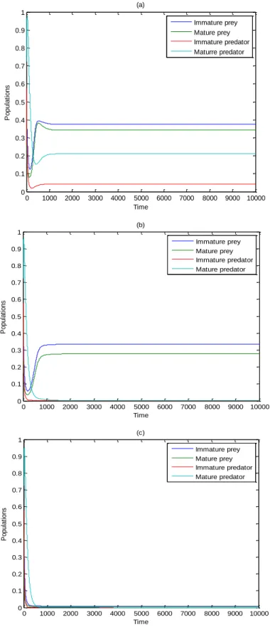
The variable the natural death velocity of the mature predator parameter and maintaining the residue of parameters’ values, as data in , it is perceived that for the resolution of Scheme leads asymptotically to the positive equilibrium point , as exhibited in Figure 1a, for conventional value while expanding this parameter for results in extermination in the predator, and the resolution of Scheme leads asymptotically to in the internal of the positive quadrant of , as exhibited in Figure 1b, for conventional value and expanding this parameter farther for 0.829 ≤ < 1 the resolution of Scheme (2) methods asymptotically to the diminishing equilibrium point as exhibited in Figure 1c, for conventional value
0 1000 2000 3000 4000 5000 6000 7000 8000 9000 10000 0 0.1 0.2 0.3 0.4 0.5 0.6 0.7 0.8 0.9 1 Time P o p u la ti o n s (a) Immature prey Mature prey Immature predator Maturre predator 0 1000 2000 3000 4000 5000 6000 7000 8000 9000 10000 0 0.1 0.2 0.3 0.4 0.5 0.6 0.7 0.8 0.9 1 Time P o p u la ti o n s (b) Immature prey Mature prey Immature predator Mature predator 0 1000 2000 3000 4000 5000 6000 7000 8000 9000 10000 0 0.1 0.2 0.3 0.4 0.5 0.6 0.7 0.8 0.9 1 Time P o p u la ti o n s (c) Immature prey Mature prey Immature predator Mature predator
Figure 1. (a): Time series of the resolution of Scheme for the data, as a result of with which leads
to in the internal of : Time series of the resolution of Scheme for the data,
as a result of with which leads to in the internal of the positive quadrant of
; and (c): Time series of the resolution of Scheme (2) for the data, as a result of (4) with , which leads to in the internal of
II. C
ONCLUSION ANDD
ISCUSSIONIn this work, the provisions of the incident of the local bifurcation were considered to study,
such assaddle-node, transcritical, and pitchfork for a mathematical model, consisting of stage-structured in prey, as well asthe predator andprey refuge. Lotka-Volterra sort of functional
rejoinder was suggested. After the investigation and analysis, it is perceived that the transcritical bifurcation transpires nearby the equilibrium point in addition to the incident of the saddle-node bifurcation at equilibrium points and . It is merit to state here that there is no likelihood incident of the pitchfork bifurcation atevery point. In conclusion, Scheme (2) was resolved numerically for the theoretical set of the parameter assigned in Equation (4) and distinctive sets of the primary point. Also, the subsequent observations are attained:
1. Changing the single parameter every time, it is perceived that changing the parameter values,
does not have any consequence on the dynamic behavior of Scheme (2), and the resolution of the scheme still approximates to the positive equilibrium point 2. As the parameter amplifying to 0.55 and maintaining the residue of parameters, as in Equation (4), the resolution of Scheme (2) approximates to the positive equilibrium point . Nevertheless, if , then, the predator will face extermination, and the trajectory will transport from the positive equilibrium point to the equilibrium point . Supplementary, if the resolution of Scheme (2) approximates to the diminishing equilibrium point ; thus, the parameters are bifurcation points of Scheme (2).
3. As the intensifying to 0.19 andretaining the remainder of parameters, as in Equation (4), the resolution of Scheme (2) approximates to the freepredator equilibrium point , whereas for the values ; then, the trajectory shifted from the free predator equilibrium point
to , which
incomes the resuscitation of the predator populace. Therefore, when
is a bifurcation point of Scheme (2). 4. As the parameter enlarging to 0.254 and maintaining the remaining parameters, as in Equation (4), the solution of Scheme (2) approaches to the positive equilibrium point further enlarging , in the range causes the predator to face extinction and the trajectory to transfer from the positive equilibrium points to the free predator equilibrium point , thus, the parameter when = 0.255 is a bifurcation point of Scheme (2).
5. As the parameter varying in the range and maintaining the rest
of parameters values, as the given data in Equation , the solution of Scheme (2) approaches asymptotically to the positive equilibrium point , while the increase of this parameter, in the ranges causes the extinction of the predator population and the transferring of trajectory
from , to ;
thus, the parameter when = 0.74 is a bifurcation point of Scheme (2).